Variational Inference and Monte Carlo Sampling are currently the two chief ways of doing approximate Bayesian inference. In the Bayesian setting, we typically have some observed variables $x$ and unobserved variables $z$, and our goal is to calculate $P(z|x)$. In all but the simplest cases, calculating $P(z|x)$ for all values of $z$ in closed form is impossible, so approximations must be made.

Variational Inference's approximation is made by choosing a family of distributions $q(z|\eta)$ parameterized by $\eta$ and choosing a setting for $\eta$ that brings $q(z|\eta)$ "close" to $P(z|x)$. In particular, Variational Inference is about finding,

$$ \begin{align*} & \arg\min_{\eta} KL \left[ q(z|\eta) || P(z|x) \right] \\ & = \arg\min_{\eta} \sum_{z} q(z|\eta) \log \frac{ q(z|\eta) }{ P(z|x) } \end{align*} $$

Looking at this formulation, the first thing you should be thinking is, "We don't even know how to calculate $P(z|x)$ much less take an expectation with respect to it. How can I possibly solve this problem?" The key is to restrict $q(z|\eta)$ to decompose into a product of independent distributions, 1 for each hidden variable $z_i$. In other words,

$$ q(z|\eta) = \prod_{i} q(z_i | \eta_i) $$

This is the "mean field approximation" and will allow us to optimize each $\eta_i$ one at a time. The final key $P(z_i|z_{-i},x)$ must lie in the exponential family, and that $q(z_i|\eta_i)$ be of the same form. For example, if the former is a Dirichlet distribution, so should the latter. When this is the case, we can solve the Coordinate Ascent update in closed form.

When all 3 conditions are met -- the mean field approximation, the univariate posteriors lie in the exponential family, and that the individual variational distributions match -- we can apply Coordinate Ascent to minimize the KL-divergence between the mean field distribution and the posterior.

Derivation of the Objective

The original intuition for Variational Inference stems from lower bounding the marginal likelihood of the observed variables $P(x)$, then maximizing that lower bound. For many choices of $q(z|\eta)$ doing this will be computationally infeasible, but we'll see that if we make the mean field approximation and choose the right variational distributions, then we can efficiently do Coordinate Ascent.

First, let's derive a lower bound on the likelihood of the observed variables,

$$ \begin{align*} \log P(x) & = \log \left( \sum_{z} P(x, z) \frac{ q(z | \eta) } { q(z | \eta) } \right) \\ & = \log \left( P(x) \sum_{z} q(z | \eta) \frac{ P(z | x) } { q(z | \eta) } \right) \\ & = \log \left( \sum_{z} q(z | \eta) \frac{ P(z | x) } { q(z | \eta) } \right) + \log P(x) \\ \end{align*} $$

Since $\log$ is a concave function, we can apply Jensen's inequality to see that $\log(p x + (1-p)y) \ge p \log(x) + (1-p) \log y$ for any $p \in [0, 1]$.

$$ \begin{align*} \log P(x) & = \log \left( \sum_{z} q(z | \eta) \frac{ P(z | x) } { q(z | \eta) } \right) + \log P(x) \\ & \ge \sum_{z} q(z | \eta) \log \left( \frac{ P(z | x) } { q(z | \eta) } \right) + \log P(x) \\ & = - \sum_{z} q(z | \eta) \log \left( \frac{ q(z | \eta) } { P(z | x) } \right) + \log P(x) \\ & = - \text{KL}[ q(z | \eta) || P(z | x) ] + \log P(x) \\ & = - \text{KL}[ q(z | \eta) || P(z , x) ] \\ \end{align*} $$

From this expression, we can see that minimizing the KL divergence over $\eta$, we're lower bounding the likelihood of the observed variables. In addition, if $q(z|\eta)$ has the same form as $P(z|x)$, then the best choice for $\eta$ is one that lets $q(z|\eta) = P(z|x)$ for all $z$.

At this point, we still have an intractable problem. Even evaluating the KL divergence requires taking an expectation over all settings for $z$ (an exponential number in $z$'s length!), so applying an iterative algorithm to choose $\eta$ is right out. However, we'll soon see that by restricting the form of $q(z|\eta)$, we can potentially decompose the KL divergence into more easily manageable bits.

The Mean Field Approximation

The key to avoiding the massive sum of the previous equation is to assume that $q(z|\eta)$ decomposes into a product of independent distributions. This is known as the "Mean Field Approximation". Mathematically, the approximation means that,

$$ q(z|\eta) = \prod_{i} q(z_i | \eta_i) $$

Suppose we make this assumption and that we want to perform coordinate ascent on a single index $\eta_k$. By factoring $P(z|x) = \prod_{i=1}^{k} P(z_i | z_{1:i-1}, x)$ and dropping all terms that are constant with respect to $\eta_k$,

$$ \begin{align*} & \arg\max_{\eta_k} -KL \left[ q(z|\eta) || p(z|x) \right] + \underbrace{\log P(x)}_{\text{constant wrt $\eta_k$}} \\ & = \arg\max_{\eta_k} \sum_{z} q(z|\eta) \log P(z|x) - \sum_{z} q(z|\eta) \log q(z|\eta) \\ & = \arg\max_{\eta_k} \sum_{z} q(z|\eta) \log \left( \prod_{i} P(z_{i}|z_{1:i-1},x) \right) - \sum_{z} \left( \prod_{i} q(z_i|\eta_i) \right) \log \left( \prod_{i} q(z_i|\eta_i) \right) \\ & = \arg\max_{\eta_k} \sum_{j} \sum_{z} q(z|\eta)\log P(z_{j}|z_{1:j-1},x) - \underbrace{ \sum_{j} \sum_{z_j} q(z_j|\eta_j) \log q(z_j|\eta_j) }_{\text{only $j=k$ not const wrt. $\eta_k$}} \\ & = \arg\max_{\eta_k} \underbrace{ \sum_{j} \sum_{z_{1:j}} \left( \prod_{i \le j} q(z_i|\eta_i) \right) \log P(z_{j}|z_{1:j-1},x) }_{\text{only last $j$ contains $q(z_k|\eta_k)$}} - \sum_{z_k} q(z_k|\eta_k) \log q(z_k|\eta_k) \\ & = \arg\max_{\eta_k} \sum_{z} q(z_k|\eta_k) \underbrace{ \left( \prod_{i \ne k} q(z_i|\eta_i) \right) }_{\text{fixed wrt $\eta_k$}} \log P(z_k | z_{-k}, x) - \sum_{z_k} q(z_k|\eta_k) \log q(z_k|\eta_k) \\ & = \arg\max_{\eta_k} \mathbb{E}_{q(z|\eta)} \left[ \log P(z_k | z_{-k}, x) \right] - \mathbb{E}_{ q(z_k|\eta_k) } \left[ \log q(z_k|\eta_k) \right] \\ \end{align*} $$

At this point, we'll make the assumption that $P(z_k|z_{-k},x)$ is an exponential family distribution ($z_{-k}$ is all $z_i$ with $i \ne k$), and moreover that $q(z_k|\eta_k)$ and $P(z_k|z_{-k},x)$ lie in the same exponential family. Mathematically, this means that,

$$ \begin{align*} q(z_k|\eta_k) &= h(z_k) \exp( \eta_i^T t(z_k) - A(\eta_k) \\ P(z_k|z_{-k},x) &= h(z_k) \exp( g(z_{-k},x)^T t(z_k) - A(g(z_{-k},x)) \\ \end{align*} $$

Here $t(\cdot)$ are sufficient statistics, $A(\cdot)$ is the log of the normalizing constant, $g(\cdot)$ is a function of all other variables that determines the parameters for $P(z_k|z_{-k},x)$, and $h(\cdot)$ is some function that doesn't depend on the parameters of the distribution.

Plugging this back into the previous equation (we define it to be $L(\eta_k)$), applying the $\log$, and using the linearity property of the expectation,

$$ \begin{align*} & \arg\max_{\eta_k} && L(\eta_k) \\ = & \arg\max_{\eta_k} && \mathbb{E}_{q(z|\eta)} \left[ \log P(z_k | z_{-k}, x) \right] - \mathbb{E}_{ q(z_k|\eta_k) } \left[ \log q(z_k|\eta_k) \right] \\ = & \arg\max_{\eta_k} &&\mathbb{E}_{q(z|\eta)} \left[ \log h(z_k) + g(z_{-k},x)^T t(z_k) - A(g(z_{-k},x) \right] - \mathbb{E}_{q(z_k|\eta_k)} \left[ \log q(z_k|\eta_k) \right] \\ = & \arg\max_{\eta_k} &&\left( \underbrace{ \mathbb{E}_{q(z_k|\eta_k)} \left[ \log h(z_k) \right] }_{\text{cancels out}} + \underbrace{ \mathbb{E}_{q(z_{-k}|\eta_{-k})} \left[ g(z_{-k},x) \right]^T \mathbb{E}_{q(z_{k}|\eta_{k})} \left[ t(z_k) \right] }_{\text{$\mathbb{E}$ splits b/c $q(z_{-k}|\eta_{-k})$ and $q(z_k|\eta_k)$ are indep.}} - \underbrace{ \mathbb{E}_{q(z_{-k}|\eta_{-k})} \left[ A(g(z_{-k},x) \right] }_{\text{const wrt $\eta_k$}} \right) \\ &&& - \left( \underbrace{ \mathbb{E}_{q(z_k|\eta_k)} \left[ \log h(z_k) \right] }_{\text{cancels out}} + \eta_k^T \mathbb{E}_{q(z_k|\eta_k)} \left[ t(z_k) \right] - A(\eta_k) \right) \\ = & \arg\max_{\eta_k} && \mathbb{E}_{q(z_{-k}|\eta_{-k})} \left[ g(z_{-k},x) \right]^T \left( \nabla_{\eta_k} A(\eta_k) \right) + \eta_k^T \left( \nabla_{\eta_k} A(\eta_k) \right) - A(\eta_k) \\ \end{align*} $$

On this last line, we use the property $\nabla A_{\eta_k} (\eta_k) = \mathbb{E}_{q(z_k|\eta_k)} [ t(z_k) ]$, a fact that holds for the exponential family. Finally, let's take the gradient of this expression and set it to zero to solve for $\eta_k$,

$$ \begin{align*} 0 & = \nabla_{\eta_k} L(\eta_k) \\ & = \left( \nabla_{\eta_k}^2 A(\eta_k) \right) \left( \mathbb{E}_{q(z_{-k}|\eta_{-k})} \left[ g(z_{-k},x) \right] - \eta_k \right) \\ \eta_k & = \mathbb{E}_{q(z_{-k}|\eta_{-k})} \left[ g(z_{-k},x) \right] \\ \end{align*} $$

So what is this expression? It says that in order to update $\eta_k$, we need to be able to evaluate the expected parameters for $P(z_k|z_{-k},x)$ under our approximation to the posterior $q(z_{-k}|\eta_{-k})$. How do we do this? Let's take a look at an example to make this concrete.

Example

For this part, let's take a look at the model defined by Latent Dirichlet Allocation (LDA),

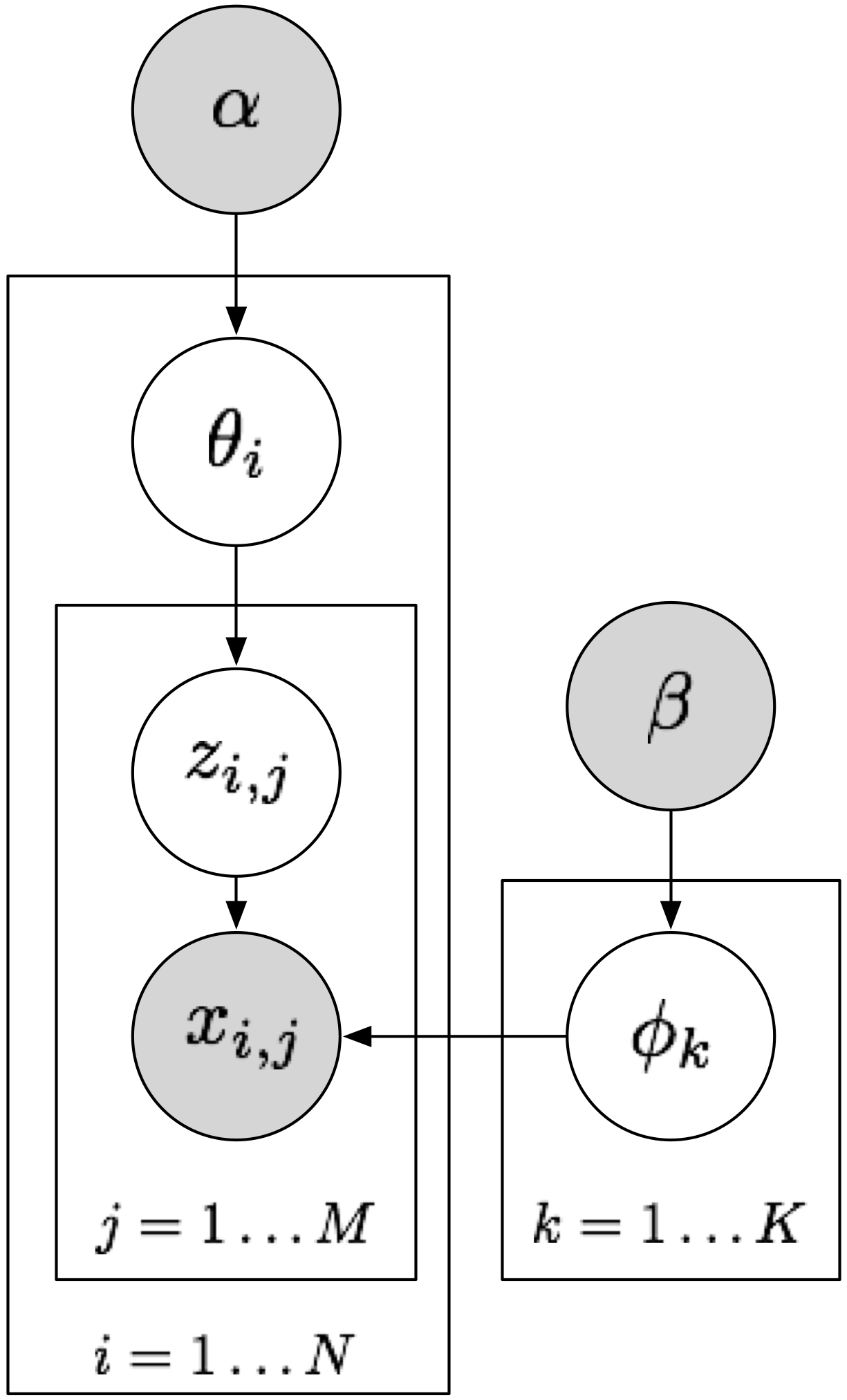
Input: document-topic prior $\alpha$, topic-word prior $\beta$

For each topic $k = 1 \ldots K$
1. Sample topic-word parameters $\phi_{k} \sim \text{Dirichlet}(\beta)$
For each document $i = 1 \ldots M$
1. Sample document-topic parameters $\theta_i \sim \text{Dirichlet}(\alpha)$
2. For each token $j = 1 \ldots N$
  1. Sample topic $z_{i,j} \sim \text{Categorical}(\theta_i)$
  2. Sample word $x_{i,j} \sim \text{Categorical}(\phi_{z_{i,j}})$

First, a short word on notation. In the following I'll occasionally drop indices to denote all variables with the same prefix. For example, when I say $\theta$, I mean $\theta_{1:M}$, and when I say $z_i$, I mean $z_{i,1:N}$. I'll also refer to $q(\theta_i|\eta_i)$ as "the variational distribution corresponding to $P(\theta_i|\alpha,\theta_{-i},z,x)$", and similarly for $q(z_{i,j}|\gamma_{i,j})$. Oh, and $z_{-i}$ means all $z_j$ with $j \ne i$, and $\theta_{1:M}$ means $(\theta_1, \ldots \theta_M)$.

Our goal now is to derive the posterior distribution over the latent variables, given the hyperparameters and the observed variables, $P(\theta, z, \phi| \alpha, x, \beta)$. We'll approximate it via the mean field distribution,

$$ q(\theta,z,\phi | \eta,\gamma,\psi) = \left( \prod_{i} q(\theta_i | \eta_i) \prod_{j} q(z_{i,j} | \gamma_{i,j}) \right) \left( \prod_{k} q(\phi_k | \psi_k) \right) $$

Outline Deriving the update rules for Variational Inference requires we do 3 things. First, we must derive the posterior distribution for each hidden variable given all other variables, hidden and observed. This distribution must lie in the exponential family, and the corresponding variational distribution for that variable must be of the same form. For example, if $P(\theta_i|\alpha,\theta_{-i},z,x)$ is a Dirichlet distribution, then $q(\theta_i|\eta_i)$ must also be Dirichlet.

Second, we need to derive, for each hidden variable, the function that gives us the parameters for the posterior distribution over that variable given all others, hidden and observed.

Finally, we'll need to plug the functions we just derived into an expectation with respect to the mean field distribution. If we are able to calculate this expectation for a particular hidden variable, we can use it to update the matching variational distribution's parameters.

In the following, I'll show you how to derive the update for the variational distribution of one of the hidden variables in LDA, $\theta_i$.

Step 1 First, we must show that the posterior distribution over each individual hidden variable lies in the exponential family. This is not always the case, but for models that employ conjugate priors, this can be guaranteed. A conjugate prior dictates that if $P(z)$ is a conjugate prior to $P(x|z)$, then $P(z|x)$ is in the same family as $P(z)$ is. This is the case for Dirichlet/Categorical distributions such as those that appear in LDA. In other words, $P(\theta_i|\alpha,\theta_{-i},z,x) = P(\theta_i|\alpha,z_{i})$ (by conditional independence) is a Dirichlet distribution because $P(\theta_i|\alpha)$ is Dirichlet and $P(z_{i,j}|\theta_i)$ is Categorical.

Step 2 Next, we derive the parameter function for each hidden variable as a function of all other variables, hidden and observed. Let's see how this plays out for the Dirichlet distribution,

The exponential family form of the Dirichlet distribution is,

$$ P(\theta_i|\alpha) = \exp \left( \sum_{k} (\alpha_k - 1) \log (\theta_i)_k - \log \left( \frac{ \prod_{k} \Gamma(\alpha_k) }{ \Gamma( \sum_k \alpha_k ) } \right) \right) $$

The exponential family form of a Categorical distribution is,

$$ P(z_{i,j}|\theta_i) = \exp \left( \sum_{k} 1[z_{i,j} = k] \log (\theta_i)_k \right) $$

Thus, the posterior distribution for $\theta_i$ is proportional to,

$$ \begin{align*} P(\theta_i|\alpha,z_{i}) & \propto P(\theta_i, z_i | \alpha) \\ & = P(\theta_i|\alpha) \prod_{j} P(z_{i,j}|\theta_i) \\ & = \exp \left( \sum_{k} \left(\alpha_k - 1 + \sum_{j} 1[z_{i,j} = k] \right) \log (\theta_i)_k \right) \end{align*} $$

Notice how $\alpha_k - 1$ changed to $\alpha_k - 1 + \sum_{j} 1[z_{i,j} = k]$? These are the parameters for our posterior distribution over $\theta_i$. Thus, the parameters for $P(\theta_i|\alpha,z_i)$ are,

$$ g_{\theta_i}(\alpha,z_{i}) = \begin{pmatrix} \alpha_1 - 1 + \sum_{j} 1[z_{i,j} = 1] \\ \alpha_2 - 1 + \sum_{j} 1[z_{i,j} = 2] \\ \vdots \\ \end{pmatrix} $$

Step 3 Now we need to take the expectation over the parameter function we just derived with respect to the mean field distribution. For $g_{\theta_i}(\alpha, z_i)$, this is particularly easy -- all the indicators simply turn into probabilities. Thus the update for $q(\theta_i|\eta_i)$ is,

$$ \eta_i = E_{q(z_{i}|\gamma_i)} [ g_{\theta_i}(\alpha, z_i) ] = \begin{pmatrix} \alpha_1 - 1 + \sum_{j} q(z_{i,j} = 1 | \gamma_{i,j}) \\ \alpha_2 - 1 + \sum_{j} q(z_{i,j} = 2 | \gamma_{i,j}) \\ \vdots \\ \end{pmatrix} $$

Conclusion We've now derived the update rule for one of the components of the mean field distribution, $q(\theta_i|\eta_i)$. Left unexplained here is the updates for $q(z_{i,j}|\gamma_{i,j})$ and $q(\phi_k|\psi_k)$, though you can find a (messier) derivation in the original paper on Latent Dirichlet Allocation.

Aside: Coordinate Ascent is Gradient Ascent

Coordinate Ascent on the Mean Field Approximation is the "traditional" way one does Variational Inference, but Coordinate Ascent is far from the only optimization method we know. What if we wanted to do Gradient Ascent? What would an update look like then?

It ends up that for the Variational Inference objective, Coordinate Ascent is Gradient Ascent with step size equal to 1. Actually, that's only half true -- it's Gradient Ascent using a "Natural Gradient" (rather than the usual gradient defined with respect to $||\cdot||_2^2$).

Gradient Ascent First, recall the Gradient Ascent update for $\eta_k$ (we use the definition of $\nabla_{\eta_k} L(\eta_k)$ we found when deriving the Coordinate Ascent update).

$$ \begin{align*} \eta_k^{(t+1)} & = \eta_k^{(t)} + \alpha^{(t)} \nabla_{\eta_k} L(\eta_k^{(t)}) \\ & = \eta_k^{(t)} + \alpha^{(t)} \left[ \left( \nabla_{\eta_k}^2 A(\eta_k^{(t)}) \right) \left( \mathbb{E}_{q(z_{-k}|\eta_{-k})} \left[ g(z_{-k},x) \right] - \eta_k^{(t)} \right) \right] \\ \end{align*} $$

Natural Gradient Hmm, that $\nabla_{\eta_k}^2 A(\eta_k^{(t)})$ term is a bit of a nuisance. Is there any way to make it just go away? In fact, we can -- by replacing the concept of a gradient with a "natural gradient". Whereas a regular gradient is the direction of steepest ascent with respect to Euclidean distance, a natural gradient is a direction of steepest ascent with respect to a function (in particular, one we want to minimize). The intuition is that for a given function, some input coordinates might be more important than others, and this should be taken into account when considering how far away 2 points are.

So what do I mean "a direction of steepest ascent"? Let's look at the gradient of a function as the solution to the following problem as $\epsilon \rightarrow 0$,

$$ \begin{align*} \nabla_{\eta_k} L(\eta_k) = & \arg\min_{d \eta_k} L(\eta_k + d \eta_k) \\ & \text{s.t.} \quad ||d \eta_k||_2^2 < \epsilon \end{align*} $$

A natural gradient with respect to $L(\eta_k)$ is defined much the same way, but with $D_{E}(x,y) = || x-y ||_2^2$ replaced with another squared metric. In our case, we're going to use the symmetrized KL divergence,

$$ D_{KL}(\eta_k, \eta_k') = \text{KL} \left[ q(z_k|\eta_k) || q(z_k|\eta_k') \right] + \text{KL} \left[ q(z_k|\eta_k') || q(z_k|\eta_k) \right] $$

Swapping the squared Euclidean metric $D_{E}$ with $D_{KL}$, we have a definition for a "Natural Gradient",

$$ \begin{align*} \hat{\nabla}_{\eta_k} L(\eta_k) = & \arg\min_{d \eta_k} L(\eta_k + d \eta_k) \\ & \text{s.t.} \quad D_{KL}(\eta_k, \eta_k + d \eta_k) < \epsilon \end{align*} $$

While at first the gradient and natural gradient may seem difficult to relate, suppose that $D_{KL}(\eta_k, \eta_k + d \eta_k) = d \eta_k^T G(\eta_k) d \eta_k$ for some matrix $G(\eta_k)$. Then by plugging this into the previous optimization problem, replacing $L(\eta_k + d \eta_k)$ by its first order Taylor approximation (which holds when $\epsilon$ is small), and requiring the derivative of the problem's Lagrangian be equal to 0, we see that,

$$ \begin{align*} 0 & = \nabla_{d \eta_k} \left[ L(\eta_k + d \eta_k) + \lambda ( d \eta_k G(\eta_k) d \eta_k - \epsilon) \right] \\ & \approx \nabla_{d \eta_k} \left[ L(\eta_k) + \nabla_{\eta_k} L(\eta_k)^T (\eta_k + d \eta_k - \eta_k) + \lambda ( d \eta_k G(\eta_k) d \eta_k - \epsilon) \right] \\ & = \nabla_{\eta_k} L(\eta_k) + 2 \lambda G(\eta_k) d \eta_k \\ d \eta_k & \propto G(\eta_k)^{-1} \nabla_{\eta_k} L(\eta_k) \end{align*} $$

As $\epsilon \rightarrow 0$, $d \eta_k$ becomes $\hat{\nabla}_{\eta_k} L(\eta_k)$, resulting in $\hat{\nabla}_{\eta_k} L(\eta_k) \propto G(\eta_k)^{-1} \nabla_{\eta_k} L(\eta_k)$. In other words, we can obtain $\hat{\nabla}_{\eta_k} L(\eta_k)$ easily if we can simply compute $G(\eta_k)$. Now let's derive $G(\eta_k)$.

First, let's take the first-order Taylor approximation to $q(z|\eta_k + d \eta_k)$ and its $\log$ about $\eta_k$,

$$ \begin{align*} q(z_k|\eta_k + d \eta_k) & \approx q(z_k|\eta_k) + (\nabla q(z_k|\eta_k))^T (\eta_k + d \eta_k - \eta_k) \\ & = q(z_k|\eta_k) + q(z_k|\eta_k) (\nabla \log q(z_k|\eta_k))^T d \eta_k \\ \log q(z_k|\eta_k + d \eta_k) & \approx \log q(z_k|\eta_k) + (\nabla \log q(z_k|\eta_k))^T (\eta_k + d \eta_k - \eta_k) \\ & = \log q(z_k|\eta_k) + (\nabla \log q(z_k|\eta_k))^T d \eta_k \\ \end{align*} $$

Plugging this back into the definition of $D_{KL}$ and cancelling out terms, we get a nice expression for $G(\eta_k)$,

$$ \begin{align*} D_{KL}(\eta, \eta') & = \text{KL} \left[ q(z_k|\eta_k) || q(z_k|\eta_k + d\eta_k) \right] + \text{KL} \left[ q(z_k|\eta_k + d\eta_k) || q(z_k|\eta_k) \right] \\ & = \sum_{z} q(z|\eta_k) \log \frac{ q(z|\eta_k) }{ q(z|\eta_k+d\eta_k) } + \sum_{z} q(z|\eta_k+d\eta_k) \log \frac{ q(z|\eta_k+d\eta_k) }{ q(z|\eta_k) } \\ & = \sum_{z} \left[ q(z|\eta_k) - q(z|\eta_k+d\eta_k) \right] \left[ \log q(z|\eta_k) - \log q(z|\eta_k+d\eta_k) \right] \\ & \approx \sum_{z} \left[ q(z|\eta_k) - q(z_k|\eta_k) - q(z_k|\eta_k)(\nabla \log q(z_k|\eta_k))^T d \eta_k \right] \\ & \qquad \quad \times \left[ \log q(z|\eta_k) - \log q(z_k|\eta_k) - (\nabla \log q(z_k|\eta_k))^T d \eta_k \right] \\ & = \sum_{z} \left[ - q(z_k|\eta_k) (\nabla \log q(z_k|\eta_k))^T d \eta_k \right] \left[ - (\nabla \log q(z_k|\eta_k))^T d \eta_k \right] \\ & = d \eta_k^T \mathbb{E}_{q(z|\eta_k)} \left[ (\nabla \log q(z_k|\eta_k)) (\nabla \log q(z_k|\eta_k))^T \right] d \eta_k \\ & = d \eta_k^T G(\eta_k) d \eta_k \\ \end{align*} $$

Looking at the expression for $G(\eta_k)$, we can see that it is in fact the Fisher Information Matrix. Since we already assumed that $q(z_k|\eta_k)$ is in the exponential family, let's plug in its exponential form $q(z_k|\eta_k) = h(z_k) \exp \left( \eta_k^T t(z_k) - A(\eta_k) \right)$ and apply the $\log$ to see that we are simply taking the covariance matrix of the sufficient statistics $t(z_k)$. For exponential families, this also happens to be the second derivative of the log normalizing constant,

$$ \begin{align*} G(\eta_k) &= \mathbb{E}_{q(z_k|\eta_k)} \left[ \left( \nabla_{\eta_k} \log q(z_k|\eta_k) \right) \left( \nabla_{\eta_k} \log q(z_k|\eta_k) \right)^T \right] \\ &= \mathbb{E}_{q(z_k|\eta_k)} \left[ \left( t(z_k) - \nabla_{\eta_k} A(\eta_k) \right) \left( t(z_k) - \nabla_{\eta_k} A(\eta_k) \right)^T \right] \\ &= \mathbb{E}_{q(z_k|\eta_k)} \left[ \left( t(z_k) - \mathbb{E}_{q(z_k|\eta_k)} [t(z_k)] \right) \left( t(z_k) - \mathbb{E}_{q(z_k|\eta_k)} [t(z_k)] \right)^T \right] \\ &= \nabla_{\eta_k}^2 A(\eta_k) \\ \end{align*} $$

Finally, let's define a Gradient Ascent algorithm in terms of the Natural Gradient, rather than the regular gradient,

$$ \begin{align*} \eta_k^{(t+1)} & = \eta_k^{(t)} + \alpha^{(t)} \hat{\nabla}_{\eta_k} L(\eta_k^{(t)}) \\ & = \eta_k^{(t)} + \alpha^{(t)} G(\eta_k^{(t)})^{-1} \nabla_{\eta_k} L(\eta_k^{(t)}) \\ & = \eta_k^{(t)} + \alpha^{(t)} \left( \nabla_{\eta_k}^2 A(\eta_k^{(t)}) \right)^{-1} \left[ \left( \nabla_{\eta_k}^2 A(\eta_k^{(t)}) \right) \left( \mathbb{E}_{q(z_{-k}|\eta_{-k})} \left[ g(z_{-k},x) \right] - \eta_k^{(t)} \right) \right] \\ & = (1 - \alpha^{(t)}) \eta_k^{(t)} + \alpha^{(t)} \mathbb{E}_{q(z_{-k}|\eta_{-k})} \left[ g(z_{-k},x) \right] \\ \end{align*} $$

Look at that -- $G(\eta_k^{(t)})^{-1} = (\nabla_{\eta_k}^2 A(\eta_k))^{-1}$ perfectly cancels out $\nabla_{\eta_k}^2 A(\eta_k)$, and we're left with a linear combination of the old parameters and the parameters Coordinate Ascent would recommend. If $\alpha^{(t)} = 1$, then we just get the old Coordinate Ascent update!

Extensions

The Variational Inference method I described here, while general in concept, can only easily be applied to a very particular class models -- ones where $P(z_k | z_{-k}, x)$ is in the exponential family. This more or less means that $z_k$ be a discrete variable or that $P(z_k)$ be a conjugate prior to all other variables depending on it.

In addition, we restricted $q(z | \eta)$ to be a mean field approximation, meaning that each variable is independent with its own distribution $q(z_k | \eta_k)$. This approximation has no hope of representing any interactions between variables, and perhaps surprisingly $q(z_k|\eta_k)$ does not match the marginal distribution over $z_k$ at all. This is a common source of confusion for first-time users, and makes debugging Variational Inference algorithms rather difficult.

Third, the Coordinate Ascent algorithm described is not necessarily quick. I explained how Coordinate Ascent is really just Gradient Ascent on the natural gradient, so it's easy to ask what other methods we might be able to apply.

Here are a handful of papers that extend Variational Inference to faster optimization methods, different variational distribution, and non-conjugate models.

"Fast Variational Inference in the Conjugate Exponential Family" -- Conjugate Gradient applied to the Marginalized Variational Bound. Shows that the Marginalized Variational Bound upper bounds the typical Variational Bound and that the former also has better curvature. That means second-order optimizers like Conjugate Gradient can take larger steps and render better performance.

"Fixed-Form Variational Posterior Approximation through Stochastic Linear Regression" -- fits a (potentially) non-decomposable exponential family distribution via Linear Regression. Involves looking at KL divergence between unnormalized variational distribution and joint distribution of model, taking derivative with respect to variational distribution's parameters and setting to 0, then solving for the parameters. Can be applied to non-conjugate models due to sampling for estimating expectations.

"Variational Inference in Nonconjugate Models" -- Getting away from conjugate priors via Laplace and the Delta Method.

References

The seminal work on the Natural Gradient is due to Shunichi Amari's "Natural Gradient Works Efficiently in Learning". The derivation for the natural gradient is Theorem 1. Thanks to Alexandre Passos for suggesting this and giving a short-hand intuition of the proof.

The derivation for Variational Inference and the correspondence between Coordinate Ascent and Gradient Ascent is based on the introduction to Matt Hoffman et al.'s "Stochastic Variational Inference".

Category: optimization
Tags: optimization , inference , bayesian