In 2002, Latent Dirichlet Allocation (LDA) was published at NIPS, one of the most highly regarded conferences for research loosely labeled as "Artificial Intelligence". The next 5 or so years led to a flurry of incremental model extensions and alternative inference methods, though none have achieved the popularity of their namesake.

Latent Dirichlet Allocation -- an extremely complex name for a not-so-complex idea. In this post, I will explain what the LDA model says, what it does not say, and how we as researchers should look at it.

The Model

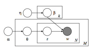
Let's begin by appreciating Latent Dirichlet Allocation in its most natural form -- the graphical model. I hope you like Greek letters...

About now, you should have an ephemeral feeling of happiness and understanding beyond anything you've ever experienced before, as if your eyes had just opened for the first time. Do you feel it? No? Yeah, I didn't think so.

Let's break it down a little, without the math. Take a look at the following 4 plots. Each subplot contains samples drawn from 1 of 3 clusters, and each plot contains samples from the same clusters. The difference between each subplot is that the number of samples from each cluster is different.

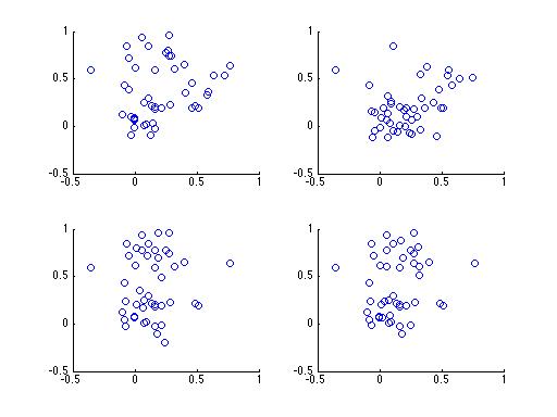
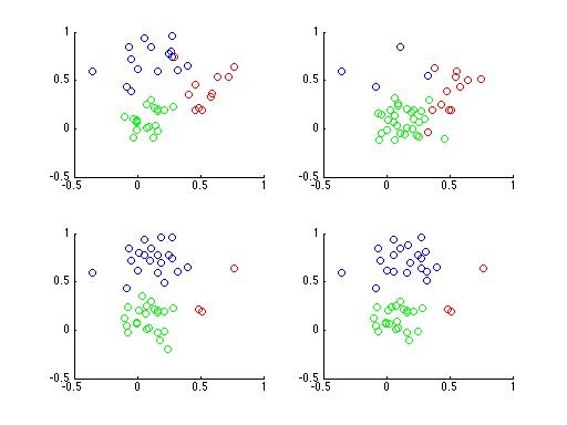
Having trouble? It's a rather difficult problem, especially with only 4 subplots. What if you had a 100,000 subplots instead? Do you think you could figure it out then? Here's a plot of the same data with points colored according to their cluster,

Even if you don't realize it yet, you now understand Latent Dirichlet Allocation. In fact, Latent Dirichlet Allocation is just an extension of the lowly Mixture Model. "How so?", you ask? Well let's look at how we might generate data from a Mixture Model.

In a mixture model, each data point is sampled independently. The algorithm for generating a sample given the model's parameters is given by the following python snippet.

def sample_mixture_model(n_data_points, cluster_weights, cluster_parameters):
  for i in range(n_data_points):
    cluster = sample_categorical(cluster_weights)
    mean, variance = cluster_parameters[cluster]
    yield sample_normal(mean, variance)

Simple, right? First, a cluster is chosen for this data point. Each cluster has some probability of being chosen, given by cluster_weights[i]. Once a cluster has been chosen, the data point is generated from a Normal distribution with mean and covariance specific to the cluster. The idea is that each cluster has its own mean and covariance, so with enough samples we'll be able to tell the clusters apart.

So how does this relate to LDA? In LDA, each "document" (in our case, subplot) is nothing more than a Mixture Model. The novel part of LDA is that there isn't just one document that we see a ton of samples from, but many documents that we only see a few samples from. Furthermore, each document has its own version of cluster_weights -- our only boon is that all documents share the same cluster_parameters.

To make that concrete, let's look at how we would generate samples from LDA.

def sample_lda(n_data_points_per_document, all_cluster_weights, cluster_parameters):
  n_documents = len(all_cluster_weights)  # number of documents
  for d in range(n_documents):
    for sample in sample_mixture_model(n_data_points_per_document,
                                       all_cluster_weights[d],
                                       cluster_parameters):
      yield {
        'document_number': d,
        'data_point': sample
      }

Notice that here we don't just return the data point by itself. In LDA, we know which "document" each data point comes from, which is just a little bit more information than we have in a regular old Mixture Model.

Finally, I have to admit that I lied a little. What I've described so far isn't quite LDA, but it's pretty damn close. In the above pseudocode, I assumed that the model parameters were already given, but LDA actually assumes the parameters are unknown and defines a probability distribution over them (a Dirichlet distribution, in fact). Secondly, the examples above generate data points from Normal distributions where as LDA generates samples from the Multinomial distribution. Other than that, you now understand Latent Dirichlet Allocation, the core of nearly every Topic Model in existence.

Appendix

Here's the MATLAB code for generating the two plots above.

%% parameters
n_samples = 200;
n_clusters = 3;
n_documents = 4;

%% reset ye olde random seed
s = RandStream('mcg16807','Seed',1);
RandStream.setDefaultStream(s);

%% generate parameters for each cluster
for i = 1:n_clusters
  mu(:,i) = rand(2,1);
  sigma(:,:,i) = rand(2,2) + 2 * eye(2);
  sigma(:,:,i) = sigma(:,:,i) + sigma(:,:,i)';
  sigma(:,:,i) = sigma(:,:,i) / 250;
end

figure;
hold on;

for d = 1:n_documents
  %% generate document-specific weights
  w = rand(n_clusters,1);
  w = w / sum(w);

  %% generate samples for this document
  for i = 1:(n_samples * rand())
    c(:,i) = mnrnd(1, w);
    z(i) = find(c(:,i));
    x(:,i) = mvnrnd(mu(:,z(i)), sigma(:,:,z(i)));
  end

  %% plotting! yay!
  subplot(2,2,d);

  % without color
  scatter(x(1,:), x(2,:));
  % with color
  % scatter(x(1,:), x(2,:), 'CData', c');
end