Convex clustering is the reformulation of k-means clustering as a convex problem. While the two problems are not equivalent, the former can be seen as a relaxation of the latter that allows us to easily find globally optimal solutions (as opposed to only locally optimal ones).

Suppose we have a set of points $\{ x_i : i = 1, \ldots, n\}$. Our goal is to partition these points into groups such that all the elements in each group are close to each other and are distant from points in other groups.

In this post, I'll talk about an algorithm to do just that.

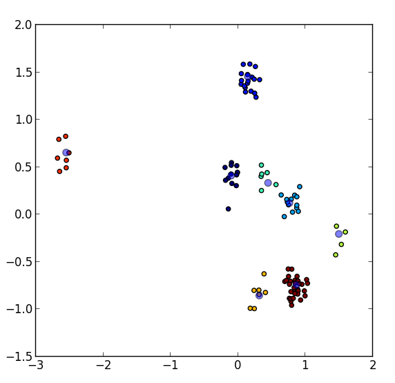8 clusters of points in 2D with their respective centers. All points of the same color belong to the same cluster.

K-Means

The original objective for k-means clustering is as follows. Suppose we want to find $k$ sets $S_i$ such that every $x_i$ is in exactly 1 set $S_j$. Each $S_j$ will then have a center $\theta_j$, which is simply the average of all $x_i$ it contains. Putting it all together, we obtain the following optimization problme,

$$ \begin{align*} & \underset{S}{\min} & & \sum_{j=1}^{k} \sum_{i \in S_j} ||x_i - \theta_j||_2^2 \\ & \text{subject to} & & \theta_j = \frac{1}{|S_j|} \sum_{i \in S_j} x_i \\ & & & \bigcup_{j} S_j = \{ 1 \ldots n \} \end{align*} $$

In 2009, Aloise et al. proved that solving this problem is NP-hard, meaning that short of enumerating every possible partition, we cannot say whether or not we've found an optimal solution $S^{*}$. In other words, we can approximately solve k-means, but actually solving it is very computationally intense (with the usual caveats about $P = NP$).

Convex Clustering

Convex clustering sidesteps this complexity result by proposing a new problem that we can solve quickly. The optimal solution for this new problem need not coincide with that of k-means, but can be seen a solution to the convex relaxation of the original problem.

The idea of convex clustering is that each point $x_i$ is paired with its associated center $u_i$, and the distance between the two is minimized. If this were nothing else, $u_i = x_i$ would be the optimal solution, and no clustering would happen. Instead, a penalty term is added that brings the clusters centers close together,

$$ \begin{align*} \min_{u} \frac{1}{2} \sum_{i=1}^{n} ||x_i - u_i||_2^2 + \gamma \sum_{i < j} w_{i,j} ||u_i - u_j||_p \end{align*} $$

Notice that the distance $||x_i - u_i||_2^2$ is a squared 2-norm, but the distance between the centers $||u_i - u_j||_p$ is a p-norm ($p \in \{1, 2, \infty \}$). This sum-of-norms type penalization brings about "group sparsity" and is used primarily because many of the elements in this sum will be 0 at the optimum. In convex clustering, that means $u_i = u_j$ for some pairs $i$ and $j$ -- in other words, $i$ and $j$ are clustered together!

Algorithms for Convex Clustering

As the convex clustering formulation is a convex problem, we automatically get a variety of black-box algorithms capable of solving it. Unfortunately, the number of variables in the problem is rather large -- if $x_i \in \mathcal{R}^{d}$, then $u \in \mathcal{R}^{n \times d}$. If $d = 5$, we cannot reasonably expect interior point solvers such as cvx to handle any more than a few thousand points.

Hocking et al. and Chi et al. were the first to design algorithms specifically for convex clustering. The former designed one algorithm for each $p$-norm, employing active sets ($p \in \{1, 2\}$), subgradient descent ($p = 2$), and the Frank-Wolfe algorithm ($p = \infty$). The latter makes use of ADMM and AMA, the latter of which reduces to proximal gradient on a dual objective.

Here, I'll describe another method for solving the convex clustering problem based on coordinate ascent. The idea is to take the original formulation, substitute a new primal variable $z_l = u_{l_1} - u_{l_2}$, then update a dual variable $\lambda_l$ corresponding to each equality constraint 1 at a time. For this problem, we can reconstruct the primal variables $u_i$ in closed form given the dual variables, so it is easy to check how close we are to the optimum.

Problem Reformulation

To describe the dual problem being maximized, we first need to modify the primal problem. First, let $z_l = u_{l_1} - u_{l_2}$. Then we can write the objective function as,

$$ \begin{align*} & \underset{S}{\min} & & \frac{1}{2} \sum_{i=1}^{n} ||x_i - u_i||_2^2 + \gamma \sum_{l} w_{l} ||z_l||_p \\ & \text{subject to} & & z_l = u_{l_1} - u_{l_2} \end{align*} $$

Chi et al. show on page 6 that the dual of this problem is then,

$$ \begin{align*} & \underset{\lambda}{\max} & & - \frac{1}{2} \sum_{i} ||\Delta_i||_2^2 - \sum_{l} \lambda_l^T (x_{l_1} - x_{l_2}) \\ & \text{subject to} & & ||\lambda_l||_{p^{*}} \le \gamma w_l \\ & & & \Delta_{i} = \sum_{l: l_1 = i} \lambda_l - \sum_{l : l_2 = i} \lambda_l \end{align*} $$

In this notation, $||\cdot||_{p^{*}}$ is the dual norm of $||\cdot||_p$. The primal variables $u$ and dual variables $\lambda$ are then related by the following equation,

$$ u_i = \Delta_i + x_i $$

Coordinate Ascent

Now let's optimize the dual problem 1 $\lambda_k$ at a time. First, notice that $\lambda_k$ will only appear in 2 $\Delta_i$ terms -- $\Delta_{k_1}$ and $\Delta_{k_2}$. After dropping all terms independent of $\lambda_k$, we now get the following problem,

$$ \begin{align*} & \underset{\lambda_k}{\min} & & \frac{1}{2} (||\Delta_{k_1}||_2^2 + ||\Delta_{k_2}||_2^2) + \lambda_k^T (x_{k_1} - x_{k_2}) \\ & \text{subject to} & & ||\lambda_k||_{p^{*}} \le \gamma w_k \\ & & & \Delta_{k_1} = \sum_{l: l_1 = k_1} \lambda_l - \sum_{l : l_2 = k_1} \lambda_l \\ & & & \Delta_{k_2} = \sum_{l: l_1 = k_2} \lambda_l - \sum_{l : l_2 = k_2} \lambda_l \end{align*} $$

We can pull $\lambda_k$ out of $\Delta_{k_1}$ and $\Delta_{k_2}$ to get,

$$ \begin{align*} ||\Delta_{k_1}||_2^2 & = ||\lambda_k||_2^2 + ||\Delta_{k_1} - \lambda_k||_2^2 + 2 \lambda_k^T (\Delta_{k_1} - \lambda_k) \\ ||\Delta_{k_2}||_2^2 & = ||\lambda_k||_2^2 + ||\Delta_{k_2} + \lambda_k||_2^2 - 2 \lambda_k^T (\Delta_{k_2} + \lambda_k) \end{align*} $$

Let's define $\tilde{\Delta_{k_1}} = \Delta_{k_1} - \lambda_k$ and $\tilde{\Delta_{k_2}} = \Delta_{k_2} + \lambda_k$ and add $||\frac{1}{2} (\tilde{\Delta_{k_1}} - \tilde{\Delta_{k_2}} + x_{k_1} - x_{k_2})||_2^2$ to the objective.

$$ \begin{align*} & \underset{\lambda_k}{\min} & & ||\lambda_k||_2^2 + 2 \frac{1}{2} \lambda_k^T (\tilde{\Delta_{k_1}} - \tilde{\Delta_{k_2}} + x_{k_1} - x_{k_2}) + ||\frac{1}{2} (\tilde{\Delta_{k_1}} - \tilde{\Delta_{k_2}} + x_{k_1} - x_{k_2})||_2^2 \\ & \text{subject to} & & ||\lambda_k||_{p^{*}} \le \gamma w_k \\ & & & \tilde{\Delta_{k_1}} = \sum_{l: l_1 = k_1; l \ne k} \lambda_l - \sum_{l : l_2 = k_1; l \ne k} \lambda_l \\ & & & \tilde{\Delta_{k_2}} = \sum_{l: l_1 = k_2; l \ne k} \lambda_l - \sum_{l : l_2 = k_2; l \ne k} \lambda_l \end{align*} $$

We can now factor the objective into a quadratic,

$$ \begin{align*} & \underset{\lambda_k}{\min} & & ||\lambda_k - \left( - \frac{1}{2}(\tilde{\Delta_{k_1}} - \tilde{\Delta_{k_2}} + x_{k_1} - x_{k_2}) \right) ||_2^2 \\ & \text{subject to} & & ||\lambda_k||_{p^{*}} \le \gamma w_k \\ & & & \tilde{\Delta_{k_1}} = \sum_{l: l_1 = k_1; l \ne k} \lambda_l - \sum_{l : l_2 = k_1; l \ne k} \lambda_l \\ & & & \tilde{\Delta_{k_2}} = \sum_{l: l_1 = k_2; l \ne k} \lambda_l - \sum_{l : l_2 = k_2; l \ne k} \lambda_l \end{align*} $$

This problem is simply a Euclidean projection onto the ball defined by $||\cdot||_{p^{*}}$. We're now ready to write the algorithm,

Input: Initial dual variables $\lambda^{(0)}$, weights $w_l$, and regularization parameter $\gamma$

Initialize $\Delta_i^{(0)} = \sum_{l: l_1 = i} \lambda_l^{(0)} - \sum_{l: l_2 = i} \lambda_l^{(0)}$
For each iteration $m = 0,1,2,\ldots$ until convergence
1. Let $\Delta^{(m+1)} = \Delta^{(m)}$
2. For each pair of points $l = (i,j)$ with $w_{l} > 0$
  1. Let $\Delta_i^{(m+1)} \leftarrow \Delta_i^{(m+1)} - \lambda_l^{(m)}$ and $\Delta_j^{(m+1)} \leftarrow \Delta_i^{(m+1)} + \lambda_l^{(m)}$
  2. $\lambda_l^{(m+1)} = \text{project}(- \frac{1}{2}(\Delta_i^{(m+1)} - \Delta_j^{(m+1)} + x_{i} - x_{j}), \{ \lambda : ||\lambda||_{p^{*}} \le \gamma w_l \}$)
  3. $\Delta_i^{(m+1)} \leftarrow \Delta_i^{(m+1)} + \lambda_l^{(m+1)}$ and $\Delta_j^{(m+1)} \leftarrow \Delta_j^{(m+1)} - \lambda_l^{(m+1)}$
Return $u_i = \Delta_i + x_i$ for all $i$

Since we can easily construct the primal variables from the dual variables and can evaluate the primal and dual functions in closed form, we can use the duality gap to determine when we are converged.

Conclusion

In this post, I introduced a coordinate ascent algorithm for convex clustering. Empirically, the algorithm is quite quick, but it doesn't share the parallelizability or convergence proofs of its siblings, ADMM and AMA. However, coordinate descent has an upside: there are no parameters to tune, and every iteration is guaranteed to improve the objective function. Within each iteration, updates are quick asymptotically and empirically.

Unfortunately, like all algorithms based on the dual for this particular problem, the biggest burden is on memory. Whereas the primal formulation requires the number of variables grow linearly with the number of data points, the dual formulation can grow as high as quadratically. In addition, the primal variables allow for centers to be merged, allowing for potential space-savings as the algorithm is running. The dual seems to lack this property, requiring all dual variables to be fully instantiated.

References

The original formulation for convex clustering was introduced by Lindsten et al. and Hocking et al.. Chi et al. introduced ADMM and AMA-based algorithms specifically designed for convex clustering.

Category: optimization
Tags: optimization , coordinate-descent , clustering

Strongly Convex

Coordinate Ascent for Convex Clustering