In the mid-1980s, Yurii Nesterov hit the equivalent of an academic home run. At the same time, he established the Accelerated Gradient Method, proved that its convergence rate superior to Gradient Descent (\(O(1/\sqrt{\epsilon})\) iterations instead of \(O(1/\epsilon)\)), and then proved that no other first-order (that is, gradient-based) algorithm could ever hope to beat it. What a boss.

Continuing my analogy, imagine that you are standing on the side of a mountain and want to reach the bottom. If you were to follow the Accelerated Gradient Method, you'd do something like this,

As we'll see, that last unintuitive bit is the key to Accelerated Gradient Descent's speed.

How does it work?

We begin by assuming the we want to minimize an unconstrained function \(f\),

As with Gradient Descent, we'll assume that \(f\) is differentiable and that we can easily compute its gradient \(\nabla f(x)\). Then the Accelerated Gradient Method is defined as,

A Small Example

We'll try out Accelerated Gradient on the same example used to showcase Gradient Descent. We'll use the objective function \(f(x) = x^4\), meaning that \(\nabla_x f(x) = 4 x^3\). For a step size, we'll use Backtracking Line Search where the largest acceptable step size is \(0.05\). Finally, we'll start at \(x^{(0)} = 1\). Compare these 2 graphs to the ones for Gradient Descent.

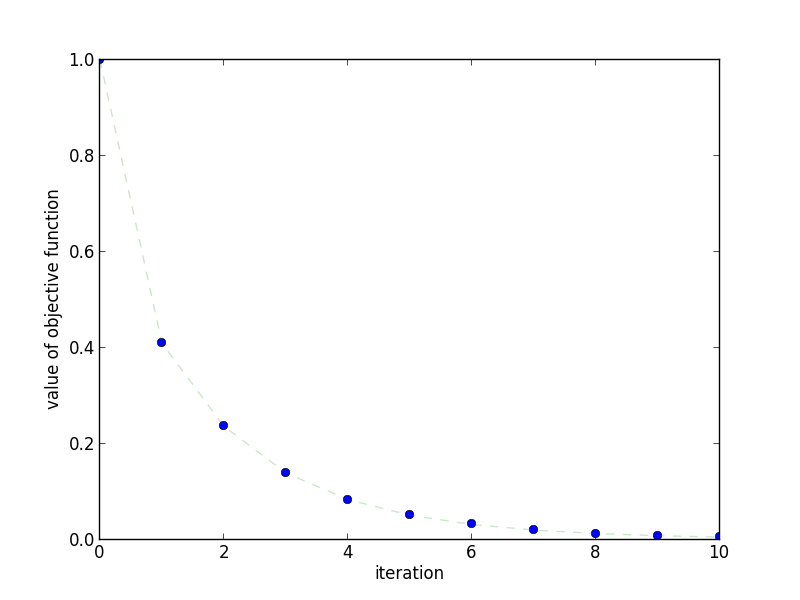This plot shows how quickly the objective function decreases as the number of iterations increases.

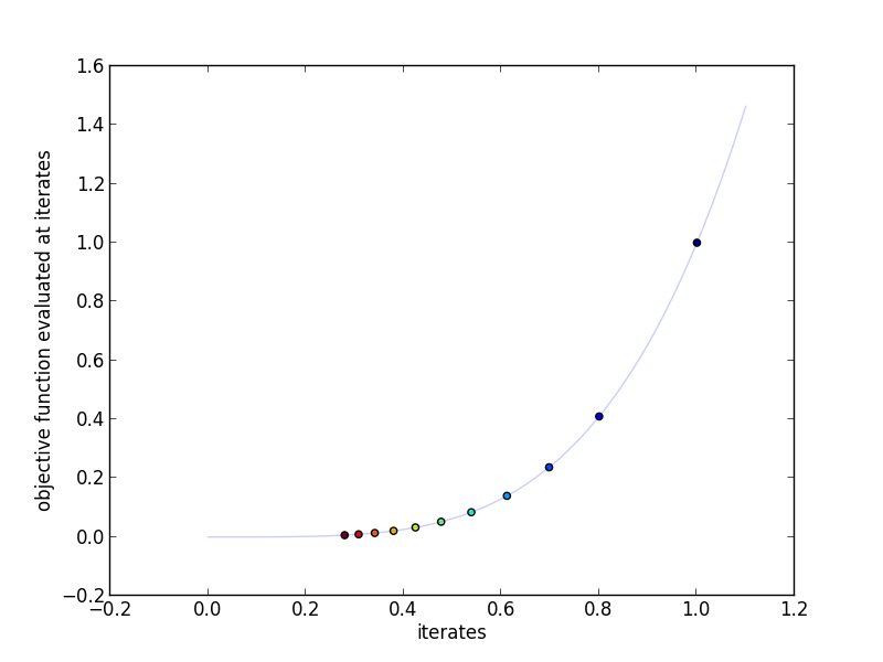This plot shows the actual iterates and the objective function evaluated at those points. More red indicates a higher iteration number.

Why does it work?

The assumptions for the Accelerated Gradient Method are identical to Gradient Descent's. In particular, we assume,

1. \(f\) is convex, differentiable, and finite for all \(x\)
2. a finite solution \(x^{*}\) exists
3. \(\nabla f(x)\) is Lipschitz continuous with constant \(L\). That is, there must be an \(L\) such that,

Assumptions As explained in my post on Gradient Descent, these assumptions give us 2 things. Assumption 1 gives us a linear lower bound on \(f\),

Assumption 3 then gives us a quadratic upper bound on \(f\),

Both of these will prove critical in the following proof.

Proof Outline The proof for the Accelerated Gradient Method is the trickiest one yet. We'll see that everything fits into place just right, but that there's very little intuition as to where it all came from.

We begin in Step 1 by defining a third iterate \(v^{(t)}\) that's a linear combination of \(x^{(t)}\) and \(x^{(t-1)}\). These iterates are purely for the sake of the proof and are not computed during the algorithm. Using these iterates, we upper bound \(f(x^{(t+1)})\) in terms of \(f(x^{(t)})\), \(f(x^{*})\), the distance between \(v^{(t+1)}\) and \(x^{*}\), and the distance between \(v^{(t)}\) and \(x^{*}\).

Step 2 involves upper bounding the error \(f(x^{(t+1)}) - f(x^{*})\) by \(f(x^{0}) - f(x^{*})\) and the distance between \(v^{(0)}\) and \(x^{*}\) using our very careful choice of \(\frac{t-1}{t+2}\).

Finally, Step 3 brings it all together by bounding \(f(x^{(t+1)}) - f(x^{*})\) by a term depending on \(1/(t+2)^2\).

Step 1 upper bounding \(f(x^{(t+1)})\). First, define the following and assume that \(\theta^{(0)} = 1\), \(v^{(0)} = x^{(0)}\),

There are 2 consequences of this definition for \(v^{(t)}\). The first is that \(y^{(t)}\) is a linear combination of \(v^{(t)}\) and \(x^{(t)}\),

The second is that \(v^{(t)}\) is a gradient step on \(v^{(t)}\), except that the gradient is evaluated at \(y^{(t)}\) (work backwards from the following),

With these 2 properties in hand, let's upper bound \(f(x^{(t)})\). Let \(\alpha^{(t)} \le \frac{1}{L}\) and define \(x^{+} \triangleq x^{(t)}\), \(x \triangleq x^{(t-1)}\), \(v^{+} \triangleq v^{(t)}\), \(v \triangleq v^{(t-1)}\), \(\alpha^{+} \triangleq \alpha^{(t)}\), \(y \triangleq y^{(t-1)}\), \(\theta \triangleq \theta^{(t-1)}\)

Using the Lipschitz assumption on \(||\nabla f(y)||_2\) and that \(\alpha^{+} \le \frac{1}{L}\),

Using convexity's linear lower bound and its line-over-function properties,

Step 2 Upper bounding \(f(x^{(t+1)}) - f(x^{*})\). We begin by manipulating the result from step 1 into something such that the left and right side look almost the same,

Remember how \(\theta^{(t)} = \frac{2}{t+2}\)? Well that means \(\theta^{(t)} > 0\) and thus \(\frac{1 - \theta^{(t)}}{ (\theta^{(t)})^2 } \le \frac{1}{ (\theta^{(t)})^2 }\). Subbing that into the previous equation lets us apply it recursively to obtain,

Step 3 Bound the error in terms of \(\frac{1}{(t+2)^2}\). Recall that \(\theta^{(0)} = 1\) and \(v^{(0)} = x^{(0)}\). Then,

Thus, the convergence rate of the Accelerated Gradient Method is \(O(\frac{1}{\sqrt{\epsilon}})\). Woo!

When should I use it?

The Accelerated Gradient Method trumps Gradient Descent in every way theoretically, but the latter is still more widely used and preferred. Why? The fact is that Accelerated Gradient is much more of a pain to implement. Whereas with Gradient Descent you can simply check if your new iterate's score is less than the previous one, Accelerated Gradient's score may increase before decreasing again. Accelerated Gradient is also extremely sensitive to step size -- if \(\alpha^{(t)}\) isn't in \((0, \frac{1}{L}]\), it will diverge. Accelerated Gradient is a powerful but fickle tool. Use it when you can, but keep Gradient Descent handy if everything is going awry.

Extensions

Step Size As mentioned previously, Accelerated Gradient is very fickle with step size. While Backtracking Line Search can and should be used when possible, it is essential that the constants be set such that \(\alpha^{(t+1)} \le \frac{1}{L}\). In other words, when,

Typically the \(\frac{1}{2}\) in the last part of the last line is traded for another constant. This will not work for Accelerated Gradient!

Checking Convergence As with Gradient Descent and Subgradient Descent, there is no real way to be certain when \(f(x^{(t)}) - f(x^{*}) < \epsilon\) without some problem-specific knowledge. Instead, it is common to stop after a fixed number of iterations or when \(||\nabla f(x^{(t)})||_2\) is small.

References

Proof of Convergence The proof of convergence is thanks to Lieven Vandenberghe's EE236c slides hosted by Zaiwen Wen.

Reference Implementation

def accelerated_gradient(gradient, y0, alpha, n_iterations=100):
  """Accelerated Gradient Method

  Parameters
  ----------
  gradient : function
      Computes the gradient of the objective function at x
  y0 : array
      initial value for x
  alpha : function
      function computing step sizes
  n_iterations : int, optional
      number of iterations to perform

  Returns
  -------
  xs : list
      intermediate values for x
  """
  ys = [y0]
  xs = [y0]
  for t in range(1, n_iterations+1):
    y = ys[-1]
    x = xs[-1]
    g = gradient(y)
    x_plus = y - alpha(y, g) * g
    y_plus = x_plus + ((t-1)/float(t+2)) * (x_plus - x)
    ys.append(y_plus)
    xs.append(x_plus)
  return xs

class BacktrackingLineSearch(object):

  def __init__(self, function):
    self.function = function
    self.alpha    = 0.05

  def __call__(self, y, g):
    f = self.function
    a = self.alpha
    while f(y - a * g) > f(y) - 0.5 * a * (g*g):
      a *= 0.99
    return a

if __name__ == '__main__':
  import os

  import numpy as np
  import yannopt.plotting as plotting

  ### ACCELERATED GRADIENT ###

  # problem definition
  function = lambda x: x ** 4     # the function to minimize
  gradient = lambda x: 4 * x **3  # its gradient
  alpha = BacktrackingLineSearch(function)
  x0 = 1.0
  n_iterations = 10

  # run gradient descent
  iterates = accelerated_gradient(gradient, x0, alpha, n_iterations=n_iterations)

  ### PLOTTING ###

  plotting.plot_iterates_vs_function(iterates, function,
                                     path='figures/iterates.png', y_star=0.0)
  plotting.plot_iteration_vs_function(iterates, function,
                                      path='figures/convergence.png', y_star=0.0)