Not far from Gradient Descent is another first-order descent algorithm (that is, an algorithm that only relies on the first derivative) is Subgradient Descent. In implementation, they are in fact identical. The only difference is on the assumptions placed on the objective function we wish to minimize, $f(x)$. If you were to follow the Subgradient Descent algorithm to walk down a mountain, it would look something like this,

Look around you and see which way points the most downwards. If there are multiple directions that are equally downwards, just pick one.
Take a step in that direction. Then repeat.

How does it work?

As before, we adopt the usual problem definition,

$$ \min_{x} \, f(x) $$

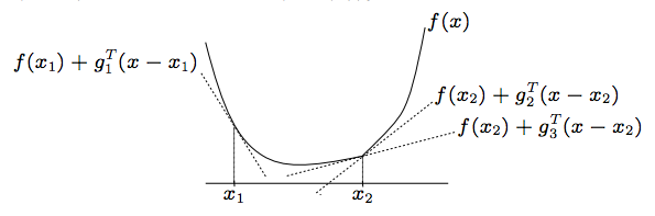
But this time, we don't assume $f$ is differentiable. Instead, we assume $f$ is convex, implying that for all $x$ there exists a $g_{x}$ such that,

$$ f(y) \ge f(x) + g_{x}^T (y - x) $$

If $f$ is differentiable at $x$ and is convex, then $\nabla f(x)$ is the only value for $g_{x}$ that satisfies this property, but if $f$ is convex but non-differentiable at $x$, there will be other options.

The set of all $g_x$ that satisfies this property called the subdifferential of $f$ at $x$ and is denoted $\partial f(x)$. Given that we have an algorithm for finding a point in the subdifferential, Subgradient Descent is

$f$ is differentiable at $x_1$, so there's only one possible subgradient (the actual gradient). At $x_2$, $f$ isn't differentiable, so $g_2$ and $g_3$ are both in $\partial f(x_2)$. Image taken from [EE392o slides][subgradient].

Input: initial iterate $x^{(0)}$

For $t = 0, 1, \ldots$
1. if converged, return $x^{(t)}$
2. Compute a subgradient of $f$ at $x^{(t)}$, $g^{(t)} \in \partial f(x^{(t)})$
3. $x^{(t+1)} = x^{(t)} - \alpha^{(t)} g^{(t)}$

The initial iterate $x^{(0)}$ can be selected arbitrarily, but $\alpha^{(t)}$ must be selected more carefully than in Gradient Descent. A common choice is $\frac{1}{t}$.

A Small Example

Let's watch Subgradient Descent do its thing. We'll use $f(x) = |x|$ as our objective function, giving us $sign(x)$ as a valid way to compute subgradients. We'll use the Polyak Step Size and initialize with $x^{(0)} = 0.75$.

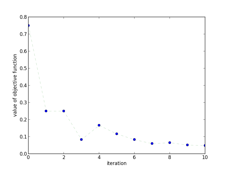This plot shows how the objective value changes as the number of iterations increase. We can see that, unlike Gradient Descent, it isn't strictly decreasing. This is expected!

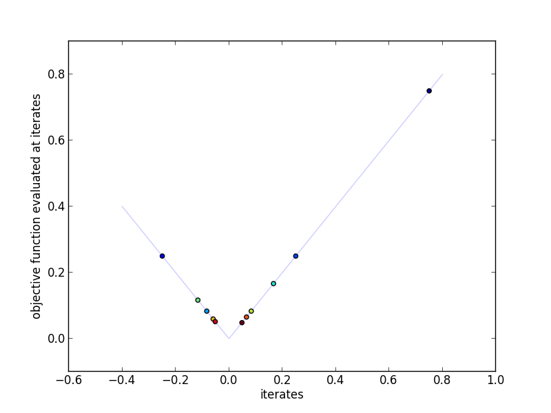This plot shows the actual iterates and the objective function evaluated at those points. More red indicates a higher iteration number.

Why does it work?

Now let's prove that Subgradient Descent can find $x^{*} = \arg\min_x f(x)$. We begin by making the following assumptions,

$f$ is convex and finite for all $x$
a finite solution $x^{*}$ exists
$f$ is Lipschitz with constant $G$. That is,

$$ || f(x) - f(y) ||_2 \le G || x - y ||_2 \qquad \forall x,y $$

The initial distance to $x^{*}$ is bounded by $R$

$$ || x^{(0)} - x^{*} || \le R $$

Assumptions Looking back at the convergence proof of Gradient Descent, we see that the main difference is in assumption 3. Before, we assumed that the $\nabla f$ was Lipschitz, but now we assume that $f$ is Lipschitz. The reason for this is because non-smooth functions cannot have a Lipschitz Subgradient function (Imagine 2 different subgradients for $f$, $g_x$ and $g_y$, such that $g_x \ne g_y$ and $x = y$. Then $||x-y||_2 = 0$ but $||g_x - g_y||_2 > 0$). However, this assumption does guarantee one thing: that $g_x \le G$ for all $x$.

Assumption 4 isn't really a condition at all. It's just a notational convenience for later.

Proof Outline The proof for Gradient Descent relied on $f(x^{(t)}) - f(x^{*})$ decreasing with each iteration, but the proof for Subgradient Descent relies on decreasing the (upper bound on) Euclidean distance between $x^{(t)}$ and the set of all possible $x^{*}$.

We begin by upper bounding the current distance to the optimal point by the previous distance ($||x^{(t)} - x^{*}||_2$), the previous error ($f(x^{(t)}) - f(x^{*})$), and the norm of the subgradient ($||g^{(t)}||_2$). Next, we recursively apply the previous finding across all $t$ to bound the sum of errors by the initial distance to $x^{*}$ and the sum of all subgradient norms. Then, we lower bound the sum of all errors with a minimum over $t$, giving us an upper bound on our error at iteration $t+1$. Finally, we use Assumption 4. to make that bound go to zero.

Step 1 Upper bound $||x^{(t+1)} - x^{*}||$. Let $x^{*}$ be any point in $\arg\min_{x} f(x)$. Then,

$$ \begin{align*} ||x^{(t+1)} - x^{*}||_2^2 = & ||x^{(t)} - \alpha^{(t)} g^{(t)} - x^{*}||_2^2 && \text{# Definition of $x^{(t+1)}$} \\ = & ||x^{(t)} - x^{*}||_2^2 - 2 \alpha^{(t)} \langle g^{(t)}, x^{(t)} - x^{*} \rangle + ( \alpha^{(t)} )^2 ||g^{(t)}||_2^2 \\ \le & ||x^{(t)} - x^{*}||_2^2 - 2 \alpha^{(t)} ( f(x^{(t)}) - f(x^{*}) ) + ( \alpha^{(t)} )^2 ||g^{(t)}||_2^2 \\ \end{align*} $$

Our last step uses $f(x^{*}) \ge f(x^{(t)}) + \langle g^{(t)}, x^{*} - x^{(t)} \rangle$

Step 2 Upper bound $||x^{(t+1)} - x^{*}||$ by $||x^{(0)} - x^{*}||$. First, we apply Step 1 recursively to bound the current distance to $x^{*}$

$$ \begin{align*} ||x^{(t+1)} - x^{*}||_2^2 \le & ||x^{(t)} - x^{*}||_2^2 - 2 \alpha^{(t)} ( f(x^{(t)}) - f(x^{*}) ) + ( \alpha^{(t)} )^2 ||g^{(t)}||_2^2 \\ \le & \left( ||x^{(t-1)} - x^{*}||_2^2 - 2 \alpha^{(t-1)} ( f(x^{(t-1)}) - f(x^{*}) ) + ( \alpha^{(t-1)} )^2 ||g^{(t-1)}||_2^2 \right) \\ & \quad - 2 \alpha^{(t)} ( f(x^{(t)}) - f(x^{*}) ) + ( \alpha^{(t)} )^2 ||g^{(t)}||_2^2 && \text{# Apply recursion}\\ = & ||x^{(t-1)} - x^{*}||_2^2 - 2 \sum_{\tau=t-1}^{t} \alpha^{(\tau)} ( f(x^{(\tau)}) - f(x^{*}) ) + \sum_{\tau=t-1}^{t} ( \alpha^{(\tau)} )^2 ||g^{(\tau)}||_2^2 \\ \vdots \\ \le & ||x^{(0)} - x^{*}||_2^2 - 2 \sum_{\tau=0}^{t} \alpha^{(\tau)} ( f(x^{(\tau)}) - f(x^{*}) ) + \sum_{\tau=0}^{t} ( \alpha^{(\tau)} )^2 ||g^{(\tau)}||_2^2 \\ \end{align*} $$

Then we drop $||x^{(t+1)} - x^{*}||_2^2$ from the left side it's lower bounded by zero,

$$ \begin{align*} 0 \le & ||x^{(0)} - x^{*}||_2^2 - 2 \sum_{\tau=0}^{t} \alpha^{(\tau)} ( f(x^{(\tau)}) - f(x^{*}) ) + \sum_{\tau=0}^{t} ( \alpha^{(\tau)} )^2 ||g^{(\tau)}||_2^2 \\ 2 \sum_{\tau=0}^{t} \alpha^{(\tau)} ( f(x^{(\tau)}) - f(x^{*}) ) \le & ||x^{(0)} - x^{*}||_2^2 + \sum_{\tau=0}^{t} ( \alpha^{(\tau)} )^2 ||g^{(\tau)}||_2^2 \\ \end{align*} $$

Step 3 Upper bound current error. First, notice that we can lower bound the contents of the sum on the left with the minimum across $\tau$,

$$ \begin{align*} \sum_{\tau=0}^{t} \alpha^{(\tau)} ( f(x^{(\tau)}) - f(x^{*}) ) \ge & \left( \min_{\tau \in 0 \ldots t} f(x^{(\tau)}) - f(x^{*}) \right) \sum_{\tau=0}^{t} ( \alpha^{(\tau)} ) \end{align*} $$

Then divide by $2 \sum_{\tau=0}^{t} ( \alpha^{(\tau)} )$,

$$ \begin{align*} 2 \left( \min_{\tau \in 0 \ldots t} f(x^{(\tau)}) - f(x^{*}) \right) \sum_{\tau=0}^{t} ( \alpha^{(\tau)} ) \le & 2 \sum_{\tau=0}^{t} \alpha^{(\tau)} ( f(x^{(\tau)}) - f(x^{*}) ) \\ \le & ||x^{(0)} - x^{*}||_2^2 + \sum_{\tau=0}^{t} ( \alpha^{(\tau)} )^2 ||g^{(\tau)}||_2^2 \\ \left( \min_{\tau \in 0 \ldots t} f(x^{(\tau)}) \right) - f(x^{*}) \le & \frac{ ||x^{(0)} - x^{*}||_2^2 + \sum_{\tau=0}^{t} ( \alpha^{(\tau)} )^2 ||g^{(\tau)}||_2^2 }{ 2 \sum_{\tau=0}^{t} ( \alpha^{(\tau)} ) } \\ \left( \min_{\tau \in 0 \ldots t} f(x^{(\tau)}) \right) - f(x^{*}) \le & \frac{ R^2 + G^2 \sum_{\tau=0}^{t} ( \alpha^{(\tau)} )^2 }{ 2 \sum_{\tau=0}^{t} ( \alpha^{(\tau)} ) } \\ \end{align*} $$

Step 4 Making the bound go to zero. Let $\alpha^{(\tau)} = \frac{R}{G \sqrt{t}}$ (this is the minimizer of the right hand side for constant $\alpha^{(\tau)}$). Then,

$$ \begin{align*} \left( \min_{\tau \in 0 \ldots t} f(x^{(\tau)}) \right) - f(x^{*}) \le & \frac{ R^2 + G^2 \sum_{\tau=0}^{t} ( \alpha^{(\tau)} )^2 }{ 2 \sum_{\tau=0}^{t} ( \alpha^{(\tau)} ) } \\ = & \frac{ R^2 + G^2 \frac{R^2}{G^2} \sum_{\tau=0}^{t} \frac{1}{t+1} }{ 2 \frac{R}{G} \sum_{\tau=0}^{t} \frac{1}{\sqrt{t+1}} } \\ = & \frac{ RG }{ 2 \sqrt{t+1} } + \frac{ RG } { 2 \sqrt{t+1} } = \frac{ RG }{ \sqrt{t+1} } \end{align*} $$

Thus, we can conclude that if we want $f(x^{(t)}) - f(x^{*}) \le \epsilon$, we need $O(\frac{1}{\epsilon^2})$ iterations. Compared to Gradient Descent's $O(\frac{1}{\epsilon})$ convergence rate, Subgradient Descent looks pretty bad!

When should I use it?

As the implementation of Gradient Descent and Subgradient Descent are essentially the same, ease of use is always the first reason to use Subgradient Descent. Similarly, Subgradient Descent requires a minimal memory footprint, and has thus found a large following in the large scale machine learning community.

As far as black box, first-order for non-differentiable convex problems go, it can be shown that Subgradient Descent is as (asymptotically) fast as we can hope for. That doesn't mean Subgradient Descent is as fast as you can get for your specific problem. Proximal Gradient methods, for example, are one such family of algorithms that allow you to exploit the properties of differentiable problems even if your problem isn't.

Extensions

Step Size As stated previously, a common choice of step size is $\alpha^{(t)} = \frac{1}{t}$, but that's far from your only choice. Indeed, any step rule that satisfies the following conditions works when inserted into the above proof,

$$ \sum_{t=0}^{\infty} \alpha^{(t)} = \infty \qquad \sum_{t=0}^{\infty} ( \alpha^{(t)} )^2 < \infty $$

For example, $\alpha^{(t)} = \frac{a}{b + t^{c}}$ for positive constants $a$ and $b$ and $c \in (0.5, 1]$ also works. These conditions are referred to as being square-summable but not summable.

If $f(x^{*})$ is known ahead of time, another choice is Polyak's Step Size,

$$ \alpha^{(t)} = \frac{ f(x^{(t)}) - f(x^{*}) } { ||g^{(t)}||_2^2 } $$

If $f(x^{*})$ isn't know, then $\alpha^{(t)} = \frac{ f(x^{(t)}) - f^{(t)}_{best} + \gamma^{(t)} }{ ||g^{(t)}||_2^2 }$ is also valid for $f^{(t)}_{best} = \min_{\tau \in 0\ldots t} f(x^{(t)})$ and $\gamma^{(t)}$ being square-summable and not summable.

Checking Convergence In short, there are no easy ways to know when to stop with Subgradient Descent. Checking if $\nabla f(x)$ is small doesn't make sense because $\nabla f(x)$ isn't defined at some points and $g_x$ doesn't necessarily get small near $x \triangleq x^{*}$. Instead, a fixed number of iterations is typically used.

References

Proof of Convergence The proof of convergence for Subgradient Descent is taken nearly verbatim from Stephen Boyd's lecture notes for EE392o course in 2003.

Polyak Step Size The algorithm for the Polyak step size was taken from page 23 of Stephen Boyd's lecture slides for EE364b.

Reference Implementation

def subgradient_descent(function, subgradient, x0, alpha, n_iterations=100):
  """Subgradient Descent

  Parameters
  ----------
  function : function
      Computes the objective function
  subgradient : function
      Computes a gradient for the objective function at x
  x0 : array
      initial value for x
  alpha : function
      function computing step sizes
  n_iterations : int, optional
      number of iterations to perform

  Returns
  -------
  xs : list
      intermediate values for x
  """
  xs = [x0]
  x_best = x0
  for t in range(n_iterations):
    x = xs[-1]
    g = subgradient(x)
    x_plus = x - alpha(t, function(x), function(x_best), g) * g
    xs.append(x_plus)
    if function(x_plus) < function(x_best):
      x_best = x_plus
  return xs


def polyak(t, f_x, f_x_best, g):
  if abs(g) > 0:
    return (f_x - f_x_best + 1.0/(t+1)) / (g * g)
  else:
    return 0.0


if __name__ == '__main__':
  import os

  import numpy as np
  import pylab as pl
  import yannopt.plotting as plotting

  ### SUBGRADIENT DESCENT ###

  function = np.abs
  subgradient = np.sign
  x0 = 0.75
  n_iterations = 10

  iterates = subgradient_descent(function, subgradient, x0, polyak, n_iterations=n_iterations)
  iterates = np.asarray(iterates)

  ### PLOTTING ###

  plotting.plot_iterates_vs_function(iterates, function,
                                     path='figures/iterates.png', y_star=0.0)
  plotting.plot_iteration_vs_function(iterates, function,
                                      path='figures/convergence.png', y_star=0.0)

Category: optimization
Tags: optimization , first-order , subgradient