When I originally wrote about the Alternating Direction Method of Multipliers algorithm, the community's understanding of its convergence properties was light to say the least. While it has long been known (See Boyd's excellent article, Appendix A) that ADMM will converge, it is only recently that the community has begun to establish how fast it converges (e.g. Hong, Deng, Feng, He).

In this article, we'll explore one way to establish an $O(1 / \epsilon)$ rate of convergence. Unlike previous convergence proofs presented in this blog, we won't directly show that the primal objective value alone converges to its optimal value; instead, we'll show that a particular function involving the primal objective and a Variational Inequality converges at the desired rate.

How does it work?

Let's begin by introducing the optimization problem ADMM solves,

$$ \begin{align} \begin{split} \underset{x,z}{\text{minimize}} \qquad & f(x) + g(z) \\ \text{s.t.} \qquad & Ax + Bz = c \\ \end{split} \label{eqn:objective} \end{align} $$

This problem is characterized by 2 primal variables, $x$ and $z$, which are related by a linear equation. In machine learning, a common scenario is to choose $A$, $B$, and $c$ such that $x = z$, making the setup particularly simple. For the rest of this article, we'll assume that $Ax + Bz = c$ is the only constraint we consider -- other constraints can be incorporated into $f$ and $g$ by letting them be infinite when constraints are broken.

The ADMM algorithm then finds the "saddle point" of the Augmented Lagrangian for the corresponding problem,

$$ \begin{align} \label{eqn:lagrangian} L_{\rho}(x, z, y) = f(x) + g(z) + \langle y, Ax + Bz - c \rangle + \frac{\rho}{2} || Ax + Bz - c ||_2^2 \end{align} $$

Note that we say Augmented Lagrangian, as the typical Lagrangian does not include the final quadratic term. It's easy to see, however, that the quadratic does not affect the problem's optimal solution, as the constraint $Ax + Bz = c$ holds for all valid solutions.

The ADMM algorithm iteratively minimizes $L_{\rho}$ with respect to $x$ for fixed $z$ and $y$, then minimizes $z$ for fixed $x$ and $y$, and finally takes a gradient step with respect to $y$ for fixed $x$ and $z$.

Input Step size $\rho$, initial primal iterates $x^{(0)}$ and $z^{(0)}$, initial dual iterate $y^{(0)}$

For $t = 0, 1, \ldots$
1. Let $x^{(t+1)} = \underset{x}{\text{argmin}} \quad L_{\rho}( x , z^{(t)}, y^{(t)} )$
2. Let $z^{(t+1)} = \underset{z}{\text{argmin}} \quad L_{\rho}( x^{(t+1)}, z , y^{(t)} )$
3. Let $y^{(t+1)} = y^{(t)} + \rho ( Ax^{(t+1)} + Bz^{(t+1)} - c )$

Intuitively, the extra quadratic term prevents each iteration of the algorithm from stepping "too far" from the last iteration, an idea that's also at the core of Proximal Gradient Descent.

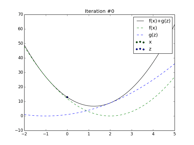Animation of $x_t$ and $z_t$ converging to the minimum of the sum of 2 quadratics.

In the remainder of the article, we'll often use the following notation for conciseness,

$$ \begin{align*} w &= \begin{bmatrix} x \\ z \\ y \end{bmatrix} \\ h(w) &= f(x) + g(z) \\ F(w) &= \begin{bmatrix} A^T y \\ B^T y \\ - (Ax + Bz - c) \end{bmatrix} \end{align*} $$

Why does it work?

Unlike other convergence proofs presented on this website, we won't directly show that the objective converges to its minimum as $t \rightarrow \infty$. Indeed, limiting ourselves to analysis of the objective completely ignores the constraint $Ax + Bz = c$. Instead, we'll use the following variational inequality condition to describe an optimal solution. In particular, a solution $w^{*}$ is optimal if,

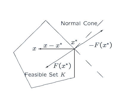$$ \begin{align} \label{vi} \forall w \in \mathbb{R}^{n} \qquad h(w) - h(w^{*}) + \langle w - w^{*}, F(w^{*}) \rangle &\ge 0 \end{align} $$

Geometric interpretation of a the optimality condition for a variational inequality when ignoring $h(w)$ from Anna Nagurney.

For the following proof, we'll replace $w^{*}$ with $\bar{w}_t = (1/t) \sum_{\tau=1}^{t} w_{\tau}$ and $0$ on the right hand side with $-\epsilon_t$ where $\epsilon_t = O(1/t)$. By showing that we can approximately satisfy this inequality at a rate $O(1/t)$, we establish the desired convergence rate.

Assumptions

The assumptions on ADMM are almost as light as we can imagine. This is largely due to the fact that we needn't use gradients or subgradients for $h(z)$.

$f(x) + g(z)$ is convex.
There exists a solution $[ x^{*}; z^{*} ]$ that minimizes $f(x) + g(z)$ while respecting the constraint $Ax + Bz = c$.

Proof Outline

The proof presented hereafter is a particularly simple if unintuitive one. Theoretically, the only tools necessary are the linear lower bound definition of a convex function, the subgradient condition for optimality in an unconstrained optimization problem, and Jensen's Inequality. Steps 1 and 2 below rely purely on the first 2 of these tools. Step 3 merely massages a preceding equation into a simpler form via completing squares. Step 4 closes by exploiting a telescoping sum and Jensen's Inequality to obtain the desired result,

$$ \forall w \qquad h(\bar{w}_t) - h(w) + \langle F(\bar{w}^{(t)}), \bar{w}^{(t)} - w \rangle \le \frac{1}{t} \left( \frac{\rho}{2} \norm{Ax-c}_2^2 + \frac{1}{2\rho} \norm{y}_2^2 \right) $$

As $t \rightarrow \infty$, the right hand side of this equation goes to 0, rendering the same statement as the variational inequality optimality condition in Equation $\ref{vi}$.

Step 1 Optimality conditions for Step A. In this portion of the proof, we'll use the fact that $x^{(t+1)}$ is defined as the solution of an optimization problem to derive a subgradient for $f$ at $x^{(t+1)}$. We'll then substitute this into $f$'s definition of convexity. Finally, terms are rearranged and the contents of Step C of the algorithm are used to derive a final expression.

We begin by recognizing that $x^{(t+1)}$ minimizes $L_{\rho}(x, z^{(t)}, y^{(t)})$ as a function of $x$. As $x$ is unconstrained, zero must be a valid subgradient for $L_{\rho}$ evaluated at $x^{(t+1)}, z^{(t)}, y^{(t)}$,

$$ \begin{align*} 0 &\in \partial_x L_{\rho}(x^{(t+1)}, z^{(t)}, y^{(t)}) \\ &= \partial_{x} f(x^{(t+1)}) + A^T y^{(t)} + \rho A^T (Ax^{(t+1)} + Bz^{(t)} - c) \\ - A^T \left( y^{(t)} + \rho (Ax^{(t+1)} + Bz^{(t)} - c) \right) &\in \partial_x f(x^{(t+1)}) \end{align*} $$

As $f$ is convex, we further know that it is lower bounded by its linear approximation everywhere,

$$ \begin{align*} \forall x \qquad f(x) &\ge f(x^{(t+1)}) + \langle \partial_x f(x^{(t+1)}), x - x^{(t+1)} \rangle \end{align*} $$

Substituting in our subgradient for $\partial_x f(x^{(t+1)})$ and subtracting the contents of the right hand side from both sides, we obtain,

$$ \begin{align*} \forall x \qquad 0 &\le f(x) - f(x^{(t+1)}) + \langle A^T (y^{(t)} + \rho (A x^{(t+1)} + B z^{(t)} - c ), x - x^{(t+1)} \rangle \end{align*} $$

Now recall Step C of the algorithm: $y^{(t+1)} = y^{(t)} + \rho (A x^{(t+1)} + Bz^{(t+1)} - c)$. The left side of the inner product looks very similar to this, so we'll substitute it in as best we can,

$$ \begin{align*} \forall x \qquad 0 &\le f(x) - f(x^{(t+1)}) + \langle A^T (y^{(t+1)} + \rho Bz^{(t)} - \rho Bz^{(t+1)}), x - x^{(t+1)} \rangle \end{align*} $$

We finish by moving everything not multiplied by $\rho$ to the opposite side of the inequality,

$$ \begin{align} \label{eqn:36} \forall x \qquad f(x^{(t+1)}) - f(x) + \langle x^{(t+1)} - x, A^T y^{(t+1)} \rangle &\le \rho \langle Bz^{(t)} - Bz^{(t+1)}, A x - A x^{(t+1)} \rangle \end{align} $$

Step 2 Optimality conditions for Step B. Similar to Step 1, we'll use the fact that $z^{(t+1)}$ is the solution to an unconstrained optimization problem and will substitute in Step C's definition for $y^{(t+1)}$.

$$ \begin{align*} 0 &\in \partial_z L(x^{(t+1)}, z, y^{(t)}) \\ &= \partial_z g(z^{(t+1)}) + B^T y^{(t)} + \rho B^T (Ax^{(t+1)} + Bz^{(t+1)} - c) \\ - B^T \left( y^{(t)} + \rho (Ax^{(t+1)} + Bz^{(t+1)} - c) \right) &\in \partial_z g(z^{(t+1)}) \end{align*} $$

As $g$ is convex, it is lower bounded by its linear approximation,

$$ \begin{align*} \forall z \qquad g(z) &\ge g(z^{(t+1)}) + \langle \partial_z g(z^{(t+1)}), z - z^{(t+1)} \rangle \end{align*} $$

Substituting in the previously derived subgradient and moving all terms to the left side, we obtain,

$$ \begin{align*} \forall z \qquad 0 &\le g(z) - g(z^{(t+1)}) + \langle B^T (y^{(t)} + \rho (A x^{(t+1)} + B z^{(t+1)} - c )), z - z^{(t+1)} \rangle \end{align*} $$

Substituting in Step C's definition for $y^{(t+1)}$ again and moving everything to the opposite side of the inequality, we conclude that,

$$ \begin{align} \label{eqn:37} \forall z \qquad g(z^{(t+1)}) - g(z) + \langle B^T y^{(t+1)}, z^{(t+1)} - z \rangle &\le 0 \end{align} $$

Step 3 We now sum Equation $\ref{eqn:36}$ with Equation $\ref{eqn:37}$. We'll end up with an expression that is not easy to understand initially, but by factoring several of its terms into quadratic forms and substituting them back in, we obtain a simpler expression that can be described as a sum of squared 2-norms.

We begin by summing equations $\ref{eqn:36}$ and $\ref{eqn:37}$.

$$ \begin{align*} & f(x^{(t+1)}) + g(z^{(t+1)}) - f(x) - g(z) + \langle B^T y^{(t+1)}, z^{(t+1)} - z \rangle + \langle A^T y^{(t+1)}, x^{(t+1)} - x \rangle \\ & \qquad \le \rho \langle Ax - Ax^{(t+1)}, Bz^{(t)} - Bz^{(t+1)} \rangle \end{align*} $$

Next, we use the definitions of $h(w)$ and $F(w)$ on the left hand side,

$$ \begin{align*} & h(w^{(t+1)}) - h(w) + \langle F(w^{(t+1)}), w^{(t+1)} - w \rangle + \langle Ax^{(t+1)} + Bz^{(t+1)} - c, y^{(t+1)} - y \rangle \\ & \qquad \le \rho \langle Ax - Ax^{(t+1)}, Bz^{(t)} - Bz^{(t+1)} \rangle \end{align*} $$

Then, moving the last term on the left side of the inequality over and observing that Step C implies $(1/\rho) (y^{(t+1)} - y^{(t)}) = Ax^{(t+1)} + Bz^{(t+1)} - c$,

$$ \begin{align} \begin{split} & h(w^{(t+1)}) - h(w) + \langle F(w^{(t+1)}), w^{(t+1)} - w \rangle \\ & \qquad \le \rho \langle Ax - Ax^{(t+1)}, Bz^{(t)} - Bz^{(t+1)} \rangle + \frac{1}{\rho} \langle y^{(t+1)} - y^{(t)}, y - y^{(t+1)} \rangle \end{split} \label{eqn:38} \end{align} $$

We will now tackle the two components on the right hand side of the inequality in isolation. Our goal is to rewrite these inner products in terms of sums of $\norm{\cdot}_2^2$ terms.

We'll start with $\langle Ax - Ax^{(t+1)}, Bz^{(t)} - Bz^{(t+1)} \rangle$. In the next equations, we'll add many terms that will cancel themselves out, then we'll group them together into a sum of 4 terms,

$$ \begin{align} & \begin{split} 2 \langle Ax - Ax^{(t+1)}, Bz^{(t)} - Bz^{(t+1)} \rangle \end{split} \notag \\ & \begin{split} = & + \norm{Ax -c}_2^2 & + 2 \langle Ax - c, B z^{(t )} \rangle & + \norm{Bz^{(t )}}_2^2 \\ & - \norm{Ax -c}_2^2 & - 2 \langle Ax - c, B z^{(t+1)} \rangle & - \norm{Bz^{(t+1)}}_2^2 \\ & + \norm{Ax^{(t+1)}-c}_2^2 & + 2 \langle Ax^{(t+1)} - c, B z^{(t+1)} \rangle & + \norm{Bz^{(t+1)}}_2^2 \\ & - \norm{Ax^{(t+1)}-c}_2^2 & - 2 \langle Ax^{(t+1)} - c, B z^{(t )} \rangle & - \norm{Bz^{(t )}}_2^2 \end{split} \notag \\ & \begin{split} = & + \norm{Ax + Bz^{(t)} - c}_2^2 & - \norm{Ax + Bz^{(t+1)} - c}_2^2 \\ & + \norm{Ax^{(t+1)} + Bz^{(t+1)} - c}_2^2 & - \norm{Ax^{(t+1)} + Bz^{(t )} - c}_2^2 \end{split} \label{eqn:39} \end{align} $$

We'll do the same for $\langle y^{(t+1)} - y^{(t)}, y - y^{(t+1)} \rangle$,

$$ \begin{align} & \begin{split} 2 \langle y^{(t+1)} - y^{(t)}, y - y^{(t+1)} \rangle \end{split} \notag \\ & \begin{split} = & + \norm{y }_2^2 & + 2 \langle y , - y^{(t )} \rangle & + \norm{y^{(t )}}_2^2 \\ & - \norm{y }_2^2 & - 2 \langle y , - y^{(t+1)} \rangle & - \norm{y^{(t+1)}}_2^2 \\ & - \norm{y^{(t)}}_2^2 & - 2 \langle y^{(t)}, - y^{(t+1)} \rangle & - \norm{y^{(t+1)}}_2^2 \\ \end{split} \notag \\ & \begin{split} = & + \norm{y - y^{(t )}}_2^2 - \norm{y - y^{(t+1)}}_2^2 - \norm{y^{(t)} - y^{(t+1)}}_2^2 \end{split} \label{eqn:40} \end{align} $$

Finally, let's plug equations $\ref{eqn:39}$ and $\ref{eqn:40}$ into $\ref{eqn:38}$.

$$ \begin{align} \begin{split} & h(w^{(t+1)}) - h(w) + \langle F(w^{(t+1)}), w^{(t+1)} - w \rangle \\ & \qquad \le \frac{\rho}{2} \left( \begin{split} & + \norm{Ax + Bz^{(t )} - c}_2^2 & - \norm{Ax + Bz^{(t+1)} - c}_2^2 \\ & + \norm{Ax^{(t+1)} + Bz^{(t+1)} - c}_2^2 & - \norm{Ax^{(t+1)} + Bz^{(t )} - c}_2^2 \end{split} \right) \\ & \qquad + \frac{1}{2\rho} \left( \begin{split} & + \norm{y - y^{(t )}}_2^2 \\ & - \norm{y - y^{(t+1)}}_2^2 \\ & - \norm{y^{(t)} - y^{(t+1)}}_2^2 \end{split} \right) \end{split} \end{align} $$

Recall that $(1/\rho)(y^{(t+1)} - y^{(t)}) = Ax^{(t+1)} + Bz^{(t+1)} - c$. Then,

$$ \begin{align*} \frac{\rho}{2} \norm{ Ax^{(t+1)} + Bz^{(t+1)} - c } &= \frac{\rho}{2} \norm{ \frac{1}{\rho} (y^{(t+1)} - y^{(t )}) } \\ &= \frac{1}{2\rho} \norm{ y^{(t )} - y^{(t+1)} } \end{align*} $$

We can substitute that into the right hand side of the preceding equation to cancel out a couple terms,

$$ \begin{align*} = & \frac{\rho}{2} \left( \begin{split} & + \norm{Ax + Bz^{(t)} - c}_2^2 & - \norm{Ax + Bz^{(t+1)} - c}_2^2 \\ & & \underbrace{- \norm{Ax^{(t+1)} + Bz^{(t )} - c}_2^2}_{ \text{ always $\le 0$ } } \end{split} \right) \\ & + \frac{1}{2\rho} \left( \begin{split} & + \norm{y - y^{(t )}}_2^2 \\ & - \norm{y - y^{(t+1)}}_2^2 \end{split} \right) \end{align*} $$

Finally dropping the portion of the equation that's always non-positive (doing so doesn't affect the validity of the inequality), we obtain a concise inequality in terms of sums of $\norm{\cdot}_2^2$.

$$ \begin{align*} & h(w^{(t+1)}) - h(w) + \langle F(w^{(t+1)}), w^{(t+1)} - w \rangle \\ & \qquad \le \frac{\rho}{2} \left( \norm{Ax + Bz^{(t )} - c}_2^2 - \norm{Ax + Bz^{(t+1)} - c}_2^2 \right) \\ & \qquad + \frac{1}{2\rho} \left( \norm{y - y^{(t )}}_2^2 - \norm{y - y^{(t+1)}}_2^2 \right) \end{align*} $$

Step 4 Averaging across iterations. We're now in the home stretch. In this step, we'll sum the previous equation across $t$. The sum will "telescope", crossing out terms until we're left only with the initial and final conditions. A quick application of Jensen's inequality will get us the desired result.

We begin by summing the previous equation across iterations,

$$ \begin{align*} & \sum_{\tau=0}^{t-1} h(w^{(\tau+1)}) - h(w) + \langle F(w^{(\tau+1)}), w^{(\tau+1)} - w \rangle \\ & \qquad \le \frac{\rho}{2} \left( \norm{Ax + Bz^{(0)} - c}_2^2 \underbrace{- \norm{Ax + Bz^{(t)} - c}_2^2}_{\le 0} \right) + \frac{1}{2\rho} \left( \norm{y - y^{(0)}}_2^2 \underbrace{- \norm{y - y^{(t)}}_2^2}_{\le 0} \right) \end{align*} $$

For convenience, we'll choose $z^{(0)}$ and $y^{(0)}$ equal to zero. We'll also drop the terms $-\norm{Ax + Bz^{(t)} - c}_2^2$ and $-\norm{y - y^{(t)}}_2^2$ from the expression, as both terms are always non-positive. This gives us,

$$ \begin{align*} \sum_{\tau=0}^{t-1} h(w^{(\tau+1)}) - h(w) + \langle F(w^{(\tau+1)}), w^{(\tau+1)} - w \rangle \le \frac{\rho}{2} \norm{Ax - c}_2^2 + \frac{1}{2\rho} \norm{ y }_2^2 \end{align*} $$

Finally, recall that for a convex function $h(w)$, Jensen's Inequality states that

$$ h(\bar{w}_t) = h \left( \frac{1}{t} \sum_{\tau=1}^{t} w_{\tau} \right) \le \frac{1}{t} \sum_{\tau=1}^{t} h(w_{\tau}) $$

The same is true for each of $F(w)$'s components (they're linear in $w$). Thus, we can apply this statement to the left hand side of the preceding equation after multiplying by $1/t$ to obtain,

$$ \begin{align*} h(\bar{w}^{(t)}) - h(w) + \langle F(\bar{w}^{(t)}), \bar{w}^{(t)} - w \rangle \le \frac{1}{t} \left( \frac{\rho}{2} \norm{Ax - c}_2^2 + \frac{1}{2\rho} \norm{ y }_2^2 \right) \end{align*} $$

The right hand side decreases as $O(1/t)$, thus ADMM converges at a rate of at least $O(1/\epsilon)$ as desired.

When should I use it?

Similar to the proximal methods presented on this website, ADMM is only efficient if we can perform each of its steps efficiently. Solving 2 optimization problems at each iteration may be very fast or very slow, depending on if a closed form solution exists for $x^{(t+1)}$ and $z^{(t+1)}$.

ADMM has been particularly useful in supervised machine learning, where $A$, $B$, and $c$ are chosen such that $x = z$. In this scenario, $f$ is taken to be the prediction loss on the training set, and $g$ an appropriate regularizer, typically a norm such as $\ell_1$ or a group sparsity norm. ADMM also lends itself to inferring the most likely setting for settings for latent variables in a factor graph. The primary benefit of ADMM in both of these cases is not its rate of convergence but how easily it lends itself to distributed computation. Applications in Compressed Sensing see similar benefits.

All in all, ADMM is not a quick method, but it is a scalable one. ADMM is best suited when data is too large to fit on a single machine or when $x^{(t+1)}$ and $z^{(t+1)}$ can be solved for in closed form. While very interesting in its own right, ADMM should rarely your algorithm of choice.

Extensions

Accelerated As ADMM is so closely related to Proximal Gradient-based methods, one might ask if there exists an accelerated variant with a better convergence rate. The answer is a resounding yes, as shown by Goldstein et al., though care must be taken for non-strongly convex objectives. In their article, Goldstein et al. show that a convergence rate of $O(1/\sqrt{\epsilon})$ can be guaranteed if both $f$ and $g$ are strongly convex. If this isn't the case, only a rate of $O(1/\epsilon)$ is shown.

Online In online learning, one is interested in solving a series of supervised machine learning instances in sequence with minimal error. At each iteration, the algorithm is presented with an input $x_t$, to which it responds with a prediction $\hat{y}_t$. The world then presents the algorithm with the correct answer $y_t$, and the algorithm suffers loss $l_t(y_t, \hat{y}_t)$. The goal of the algorithm is to minimize the sum of errors $\sum_{t} l_t(y_t, \hat{y}_t)$.

In this setting, Wang has shown that an online variant to ADMM can achieve regret competitive with the best possible ($O(\sqrt{T})$ for convex loss functions, $O(\log(T))$ for strongly convex loss functions).

Stochastic In a stochastic setting, one is interested in minimizing the average value of $f(x)$ via a series of samples. In Ouyang et al, convergence rates for a linearized variant of ADMM when $f$ can only be accessed through samples.

Multi Component Traditional ADMM considers an objective with only 2 components $f(x)$ and $g(z)$. While applying the same logic to 3 or more is straightforward, proving convergence for this scenario is more difficult. This was the task taken by He et al. In particular, they showed that a special variant of ADMM using "Gaussian back substitution" is ensured to converge.

References

ADMM While ADMM has existed for decades, it has only recently been brought to light by Boyd's article describing its applications for statistical machine learning. It is from this work from which I initially learned of ADMM.

Proof of Convergence The proof of convergence presented here is a verbose expansion of that presented in Wang's paper on Online ADMM.

Reference Implementation

Using the optim Python package, we can generate the animation above,

"""
Example usage of ADMM solver.

A gif is generated showing the iterates as they converge.
"""
from matplotlib import animation
from optim.admm import *
from optim.tests.test_admm import quadratic1
import itertools as it
import numpy     as np
import pylab as pl
import sys


if len(sys.argv) != 2:
  sys.stderr.write("Usage: %s OUTPUT\n" % (sys.argv[0],))
  sys.exit(1)
else:
  output = sys.argv[1]

prob, state = quadratic1()
admm        = ADMM(rho=0.1)
iterates    = list(it.islice(admm.solve(prob, state), 0, 50))

pl.figure()
_   = np.linspace(-2, 5)
xs  = np.asarray([s.x for s in iterates])
zs  = np.asarray([s.z for s in iterates])
xs2 = [prob.primal(State(x=v,z=v,y=0)) for v in xs]
zs2 = [prob.primal(State(x=v,z=v,y=0)) for v in zs]

def animate(i):
  print 'iteration:', i
  pl.cla()
  pl.title("Iteration #%d" % i)
  pl.plot   (_, [prob.f(v) + prob.g(v) for v in _], 'k-' , label='f(x)+g(z)')
  pl.plot   (_, [prob.f(v)             for v in _], 'g--', label='f(x)'     )
  pl.plot   (_, [            prob.g(v) for v in _], 'b--', label=     'g(z)')
  pl.scatter(xs[i], xs2[i], c='g', label='x')
  pl.scatter(zs[i], zs2[i], c='b', label='z')
  pl.xlim(min(_), max(_))
  pl.legend()

anim = animation.FuncAnimation(pl.gcf(), animate, frames=len(iterates))
anim.save(output, writer='imagemagick', fps=4)

Category: optimization
Tags: optimization , distributed , admm

Strongly Convex

ADMM revisited